1 Content
This is a set of code and data sets to document and reproduce the computational analyses in Steffen et al., 2020. In brief, it contains three parts: the metabolome, microbiota and inter-omics analyses. For the metabolome, we include detailed descriptions of the metabolomics data acquisition, data processing with xcms, and multivariate analyses with ropls. In addition, signals of known and novel compounds of interest were manually extracted and analysed. For the microbiota, we include community visualisation and ecological analyses in vegan. The inter-omics section contains mantel test and procrustes rotations, as well as the microbial interaction network annotated with the OTU’s correlation with barettin, and their response to depth.
We hope to contribute to good science by providing reproducible documentation of the computational workflow. If you have questions, comments or suggestions please feel free to get in touch.
1.1 Experimental setup
Three demosponge species Geodia barretti (n=20), Stryphnus fortis (n=15), and Weberella bursa (n=17) (Fig 1.6) were sampled in the Davis Strait between Canada and Greenland (61.147942-66.38245 Lat,-68.78077- -57.96573 Lon) from 244 m to 1467 m depth (Fig 1.1, 1.2). Temperature and salinity in situ were recorded. Sample metadata is deposited at PANGAEA.
1.1.1 Map
library(ggplot2)
library(ggmap)
library(maps)
library(mapdata)
library(marmap)
library(ggrepel)
library(sf)
library(rnaturalearth)
library(rnaturalearthdata)

sample_coords <- read.csv("data/Steffen_et_al_metadata_PANGAEA.csv", header = T, sep = ";")
sample_coords <- sample_coords[, c("Species", "unified_ID", "Latitude", "Longitude")]
sample_coords <- na.omit(sample_coords)

world <- ne_countries(scale = "medium", returnclass = "sf")
sample_map2 <- ggplot(data = world) + geom_sf() + coord_sf(xlim = c(-95, 0), ylim = c(45, 75), expand = T) + annotate("rect", xmin = -68.78077, xmax = -57.96573,
    ymin = 61.147942, ymax = 66.38245, alpha = 0.2) + geom_point(data = sample_coords, aes(x = sample_coords$Longitude, y = sample_coords$Latitude, col = Species)) +
    ggtitle("Sample map") + xlab("Longitude") + ylab("Latitude") + theme_bw() + theme(legend.position = "none")
sample_map2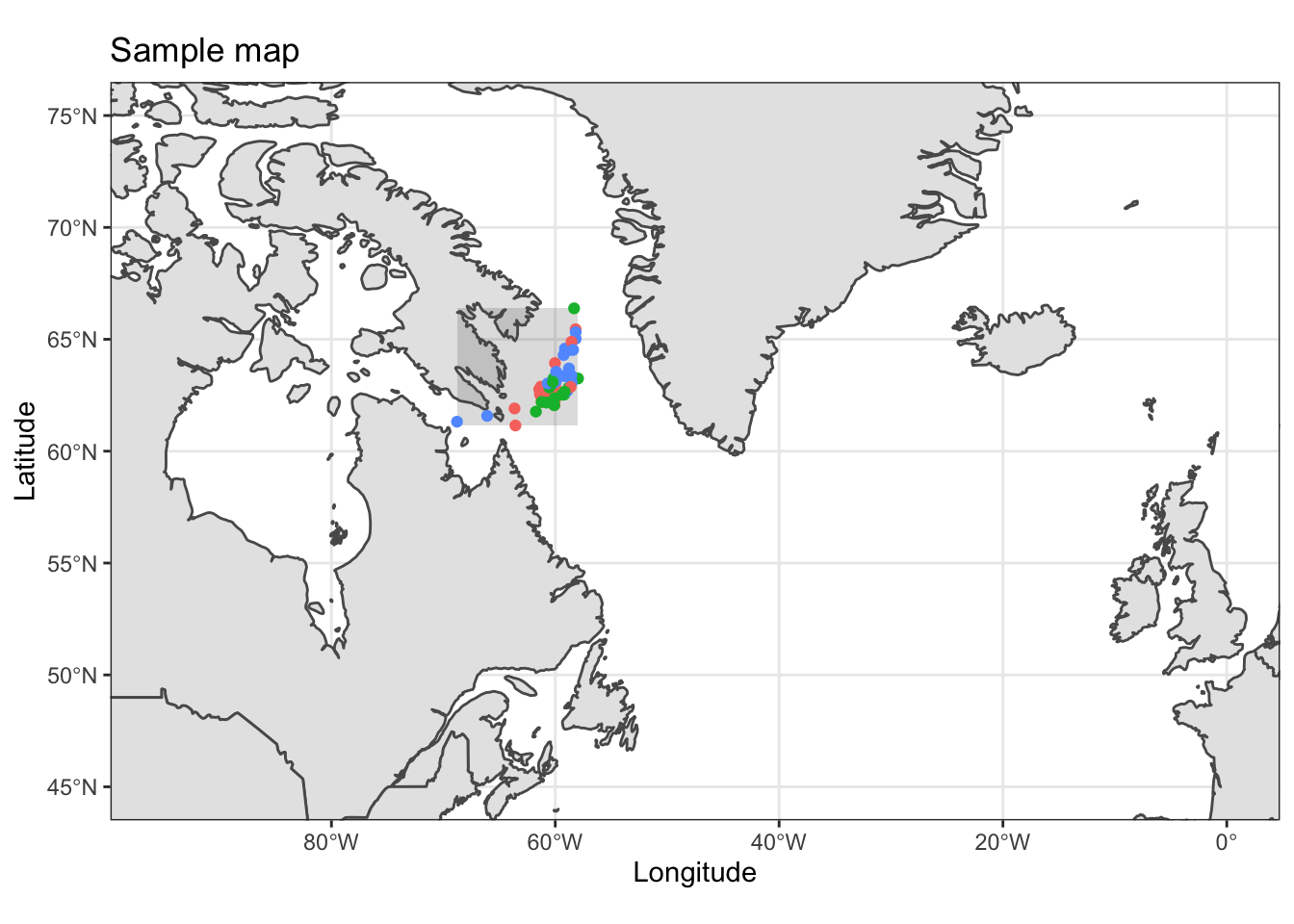
Figure 1.1: Geographic placement of the sample site on the Northern hemisphere, between Canada and Greenland. Dots indicate individual samples.
map_data <- getNOAA.bathy(-70, -50, 58, 68, resolution = 4, keep = T, antimeridian = FALSE)
sample_map_1 <- autoplot(map_data, geom = c("r", "c")) + scale_fill_gradient2(low = "dodgerblue4", mid = "gainsboro", high = "darkgreen") + geom_point(aes(x = sample_coords$Longitude,
    y = sample_coords$Latitude, colour = factor(sample_coords$Species)), data = sample_coords) + ggtitle("Sample map") + xlab("Longitude") + ylab("Latitude") +
    labs(fill = "Depth", col = "Species")
sample_map_1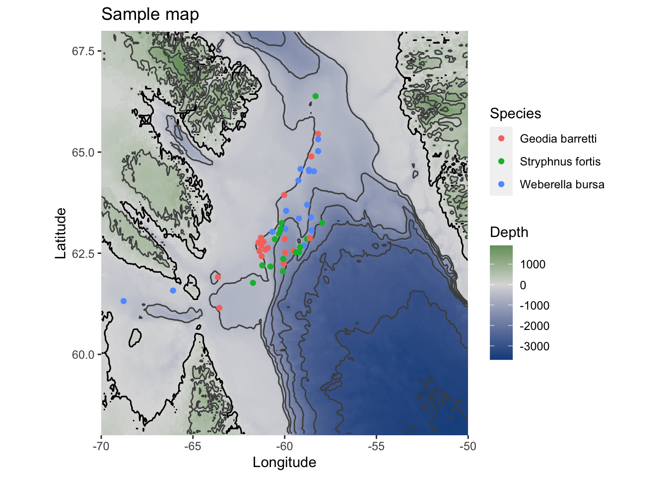
Figure 1.2: Detailed map of the sampling site, samples represented by dots are coloured according to sponge species.
# with labels: sample_map_1+geom_label_repel(aes(x=sample_coords$Longitude, y=sample_coords$Latitude, label = sample_coords$unified_ID), box.padding = 0.35,
# point.padding = 0.5, data=sample_coords)
# 3D map
library(marmap)
library(lattice) #for wireframe
map_data_hires <- getNOAA.bathy(-70, -50, 58, 68, resolution = 1, keep = T, antimeridian = FALSE)
wireframe(unclass(map_data_hires), shade = T, aspect = c(1/2, 0.1), screen = list(z = 0, x = -50), par.settings = list(axis.line = list(col = "transparent")),
par.box = c(col = rgb(0, 0, 0, 0.1)))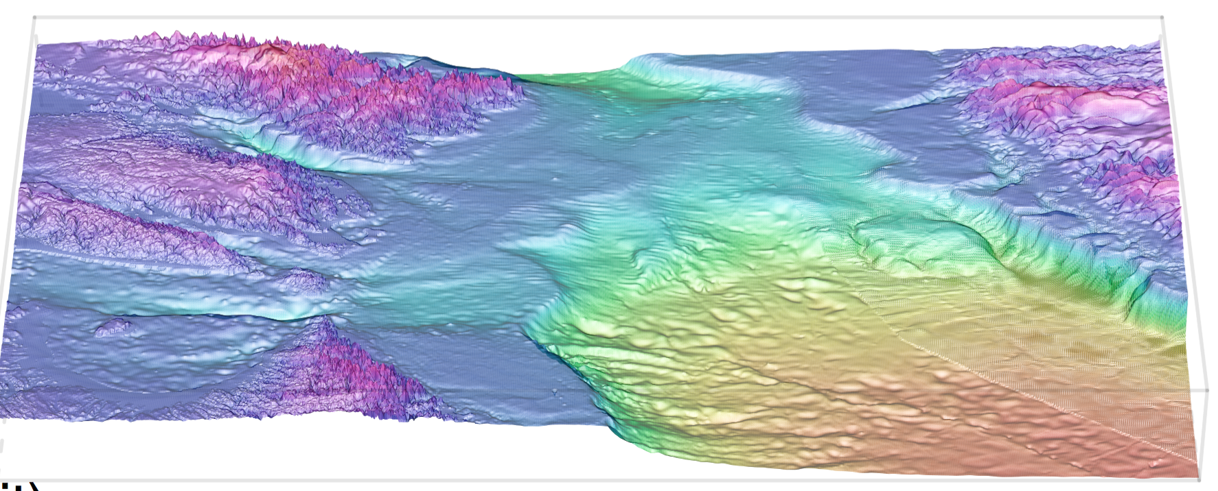
Figure 1.3: 3D representation of the threshold and slope in the Davis strait.
1.1.2 Water masses
knitr::include_graphics("data/Argo_Mean_on_Grid_Size_0dec25_2002_3-2018_6_Lambert_Lat_Range_59-65_Vector_IY20191123.png")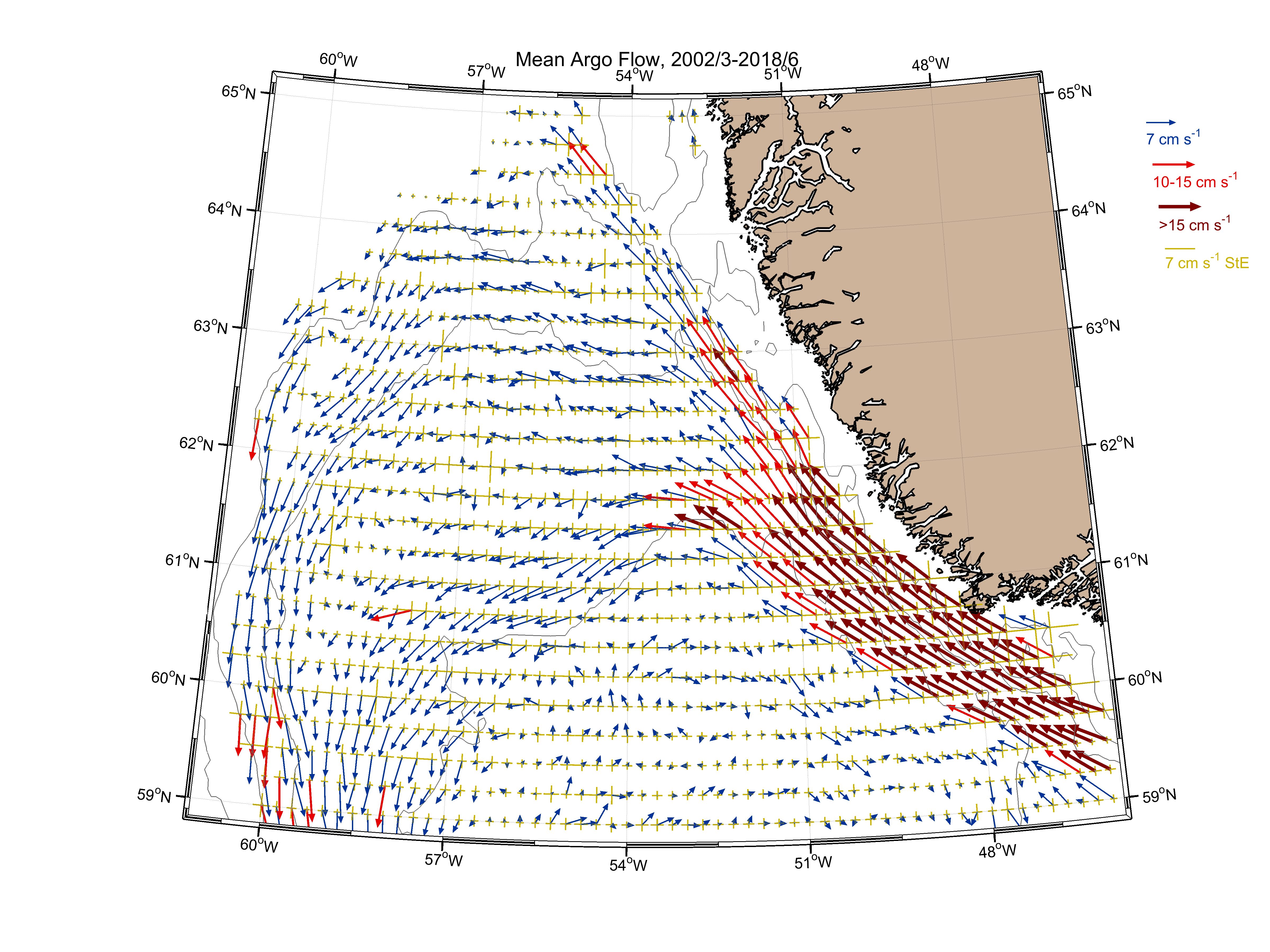
Figure 1.4: Currents in the North Atlantic between Greenland and Canada. Analysis and figure contributed by Igor Yashayaev.
knitr::include_graphics("data/water_masses_2002-2015 T-S Profiles Selected in Topo-range 300-1900 m & Colored by Depth - Labeled.png")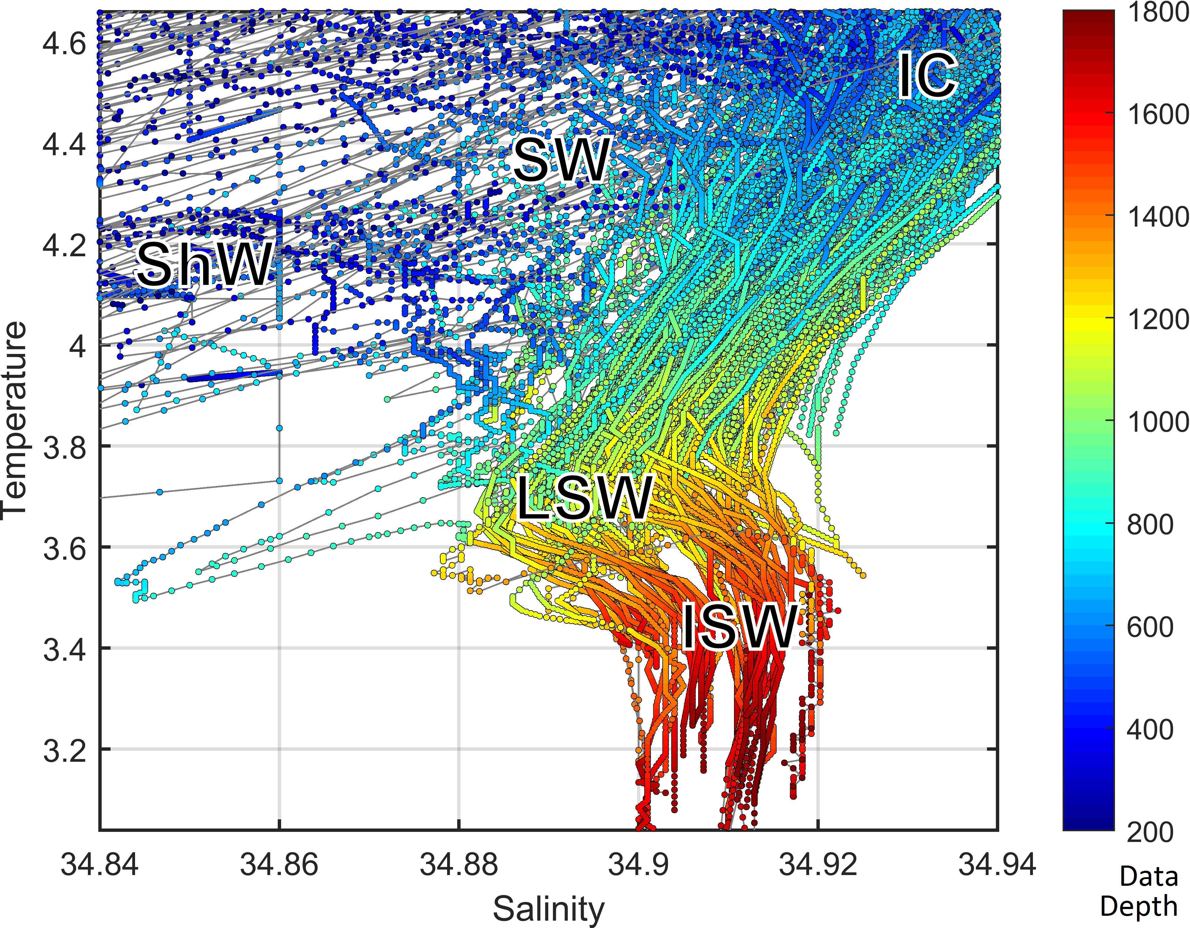
Figure 1.5: Temperature and salinity (T-S) plot showing the different water masses in the Davis strait by depth: Shelf Water (ShW), Slope Water (SW), Irminger Current (IC), Labrador Sea Water (LSW), and Icelandic slope water (ISW). Analysis and figure contributed by Igor Yashayaev.
1.1.3 Sponges
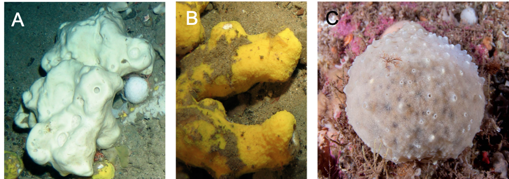
Figure 1.6: A G. barretti and B S. fortis from West Shetland Channel. Image Crown Copyright ©2006, all rights reserved. Image provided by K. Howell, Plymouth University, UK. C W. bursa, picture taken by scuba diving at 40 m in Svalbard by Peter Leopold.
G. barretti and S. fortis are high microbial abundance (HMA) sponges often found living in proximity. W. bursa is likely a low microbial abundance sponges (see diversity metrics, Nicole Boury-Esnault per.comm.). While all sponges originate from the same geographic region, W. bursa typically does not occur in the same habitats as G. barretti and S. fortis (Murillo et al. 2018). It is important to note that S. fortis is whiteish in colour, and the yellow shown in the picture stems from Hexadella dedritifera frequently found overgrowing it.
1.2 Sample metadata analysis
To investigate underlying data patterns, we assessed correlation of our predictor variables, i.e. the meta data of our samples (depth, latitude, longitude, sampling year, salinity and temperature).
1.2.1 Correlations, visual inspection and variance inflation factors (VIF) across all samples
md <- read.csv("data/Steffen_et_al_metadata_PANGAEA.csv", header = T, sep = ";")
md <- md[, c("Species", "Depth", "Latitude", "Longitude", "YEAR", "MeanBotSalinity_PSU", "MeanBottomTemp_Cdeg", "unified_ID")]

a <- cor.test(md$Depth, md$Latitude, method = "spearman")
a <- paste("Rho =", round(a$estimate, digits = 3), " p-value=", round(a$p.value, digits = 3))
b <- cor.test(md$Depth, md$Longitude, method = "spearman")
b <- paste("Rho =", round(b$estimate, digits = 3), " p-value=", round(b$p.value, digits = 3))
c <- cor.test(md$Depth, md$YEAR, method = "spearman")
c <- paste("Rho =", round(c$estimate, digits = 3), " p-value=", round(c$p.value, digits = 3))
d <- cor.test(md$Depth, md$MeanBotSalinity_PSU, method = "spearman")
d <- paste("Rho =", round(d$estimate, digits = 3), " p-value=", round(d$p.value, digits = 3))
e <- cor.test(md$Depth, md$MeanBottomTemp_Cdeg, method = "spearman")
e <- paste("Rho =", round(e$estimate, digits = 3), " p-value=", round(e$p.value, digits = 3))
f <- cor.test(md$MeanBotSalinity_PSU, md$MeanBottomTemp_Cdeg, method = "spearman")
f <- paste("T-S plot: Rho =", round(f$estimate, digits = 3), " p-value=", round(f$p.value, digits = 3))

k <- ggplot(md, aes(x = Latitude, y = Depth)) + geom_point() + scale_y_continuous(trans = "reverse") + xlab("Latitude") + ylab("Depth") + ggtitle(a) + theme(plot.title = element_text(size = 10))
l <- ggplot(md, aes(x = Longitude, y = Depth)) + geom_point() + scale_y_continuous(trans = "reverse") + xlab("Longitude") + ylab("Depth") + ggtitle(b) + theme(plot.title = element_text(size = 10))
m <- ggplot(md, aes(x = YEAR, y = Depth)) + geom_point() + scale_y_continuous(trans = "reverse") + xlab("Year") + ylab("Depth") + ggtitle(c) + theme(plot.title = element_text(size = 10))
n <- ggplot(md, aes(x = MeanBotSalinity_PSU, y = Depth)) + geom_point() + scale_y_continuous(trans = "reverse") + xlab("Salinity") + ylab("Depth") + ggtitle(d) +
    theme(plot.title = element_text(size = 10))
o <- ggplot(md, aes(x = MeanBottomTemp_Cdeg, y = Depth)) + geom_point() + scale_y_continuous(trans = "reverse") + xlab("Temperature") + ylab("Depth") + ggtitle(e) +
    theme(plot.title = element_text(size = 10))
p <- ggplot(md, aes(x = MeanBotSalinity_PSU, y = MeanBottomTemp_Cdeg, colour = md$Depth)) + geom_point(size = 2) + scale_colour_gradient(guide = guide_colourbar(),
    high = "#f4c430", low = "#3b3bc4", trans = "reverse") + xlab("Salinity in psu") + ylab("Temperature in °C") + labs(colour = "Depth") + ggtitle(f) + theme(plot.title = element_text(size = 10),
    legend.key.size = unit(0.3, "cm")) + scale_x_continuous(limits = c(34.4, 35))
# The limits of the x-axis exclude two samples from water with comparably low salinitylibrary(gridExtra)
grid.arrange(k, l, m, n, o, p, nrow = 3, top = "Spearman correlation of sample associated meta data")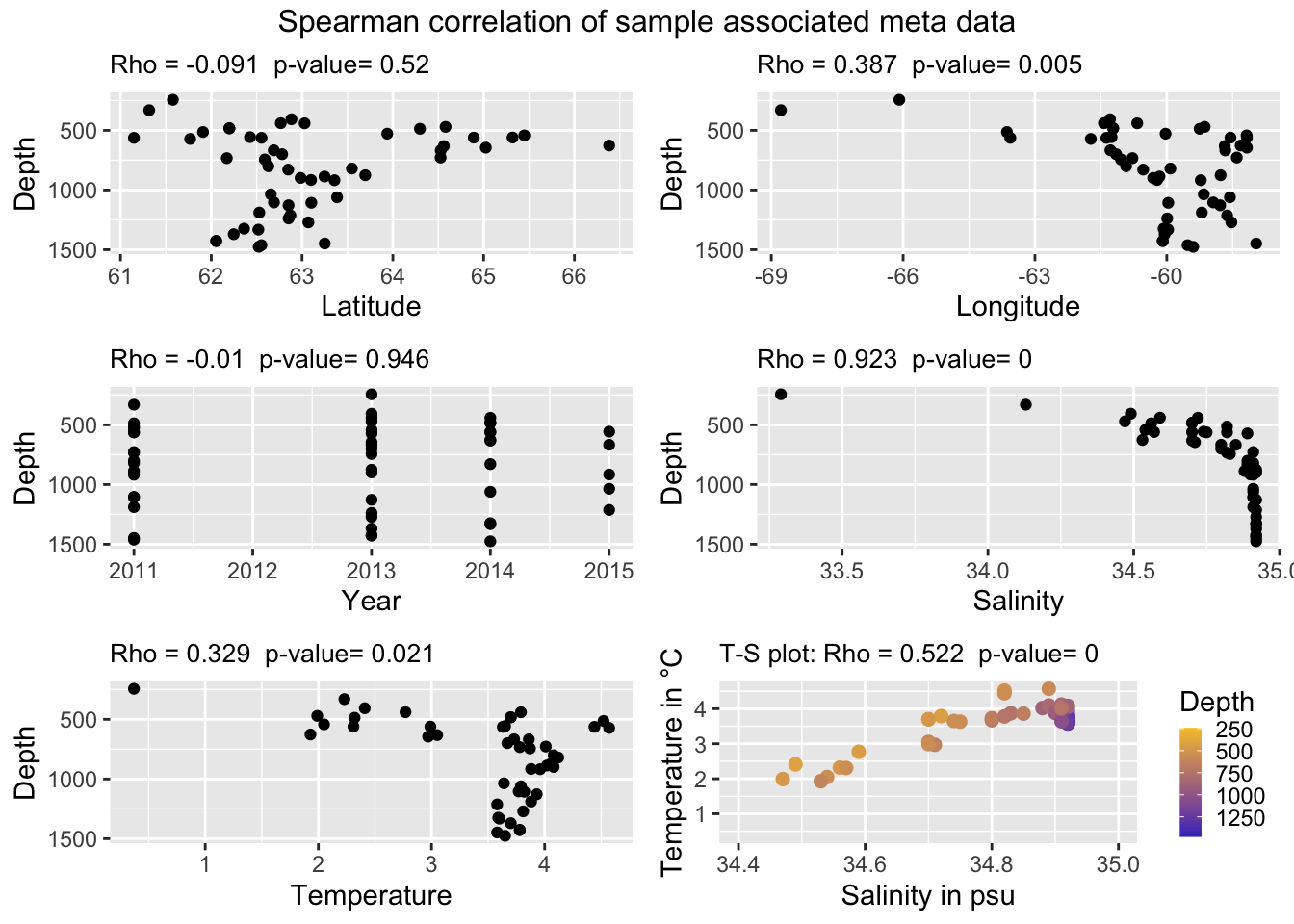
Figure 1.7: Correlation of depth with other environmental parameters/predictor variables across all samples.
In the bottom right plot showing temperature versus salinity, two samples from lower salinity were excluded for visual clarity. From the plots above and their correlation tests, we find that longitude, salinity and temperature are significantly correlated with depth, and that salinity and temperature also correlate with each other.
This is further corroborated in the variance inflation factors. A VIF > 10 indicates redundancy/collinearity. This means that we have to be cautious and avoid including redundant constraints in ecological models.
library(usdm)
md$Species <- NULL
md$unified_ID <- NULL
vif_all <- vif(md)

library(kableExtra)
options(kableExtra.html.bsTable = T)
kable(vif_all, longtable = T, booktabs = T, caption = "VIF for meta data from all samples", row.names = F) %>% kable_styling(bootstrap_options = c("striped",
"hover", "bordered", "condensed", "responsive"), full_width = F, latex_options = c("striped", "scale_down"))| Variables | VIF |
|---|---|
| Depth | 3.267983 |
| Latitude | 6.125058 |
| Longitude | 7.189093 |
| YEAR | 1.122117 |
| MeanBotSalinity_PSU | 16.131495 |
| MeanBottomTemp_Cdeg | 12.301386 |
As we will be focussing on Geodia barretti, we repeat the same inspection procedure for the sample subset.
1.2.2 Correlations, visual inspection and variance inflation factors (VIF) across G. barretti samples
md <- read.csv("data/Steffen_et_al_metadata_PANGAEA.csv", header = T, sep = ";")
md <- md[, c("Species", "Depth", "Latitude", "Longitude", "YEAR", "MeanBotSalinity_PSU", "MeanBottomTemp_Cdeg", "unified_ID")]
md <- md[md$Species == "Geodia barretti", ]

a <- cor.test(md$Depth, md$Latitude, method = "spearman")
a <- paste("Rho =", round(a$estimate, digits = 3), " p-value=", round(a$p.value, digits = 3))
b <- cor.test(md$Depth, md$Longitude, method = "spearman")
b <- paste("Rho =", round(b$estimate, digits = 3), " p-value=", round(b$p.value, digits = 3))
c <- cor.test(md$Depth, md$YEAR, method = "spearman")
c <- paste("Rho =", round(c$estimate, digits = 3), " p-value=", round(c$p.value, digits = 3))
d <- cor.test(md$Depth, md$MeanBotSalinity_PSU, method = "spearman")
d <- paste("Rho =", round(d$estimate, digits = 3), " p-value=", round(d$p.value, digits = 3))
e <- cor.test(md$Depth, md$MeanBottomTemp_Cdeg, method = "spearman")
e <- paste("Rho =", round(e$estimate, digits = 3), " p-value=", round(e$p.value, digits = 3))
f <- cor.test(md$MeanBotSalinity_PSU, md$MeanBottomTemp_Cdeg, method = "spearman")
f <- paste("Rho =", round(f$estimate, digits = 3), " p-value=", round(f$p.value, digits = 3))

k <- ggplot(md, aes(x = Latitude, y = Depth)) + geom_point() + scale_y_continuous(trans = "reverse") + xlab("Latitude") + ylab("Depth") + ggtitle(a) + theme(plot.title = element_text(size = 10))
l <- ggplot(md, aes(x = Longitude, y = Depth)) + geom_point() + scale_y_continuous(trans = "reverse") + xlab("Longitude") + ylab("Depth") + ggtitle(b) + theme(plot.title = element_text(size = 10))
m <- ggplot(md, aes(x = YEAR, y = Depth)) + geom_point() + scale_y_continuous(trans = "reverse") + xlab("Year") + ylab("Depth") + ggtitle(c) + theme(plot.title = element_text(size = 10))
n <- ggplot(md, aes(x = MeanBotSalinity_PSU, y = Depth)) + geom_point() + scale_y_continuous(trans = "reverse") + xlab("Salinity") + ylab("Depth") + ggtitle(d) +
    theme(plot.title = element_text(size = 10))
o <- ggplot(md, aes(x = MeanBottomTemp_Cdeg, y = Depth)) + geom_point() + scale_y_continuous(trans = "reverse") + xlab("Temperature") + ylab("Depth") + ggtitle(e) +
    theme(plot.title = element_text(size = 10))
p <- ggplot(md, aes(x = MeanBotSalinity_PSU, y = MeanBottomTemp_Cdeg, colour = md$Depth)) + geom_point(size = 2) + scale_colour_gradient(guide = guide_colourbar(),
    high = "#f4c430", low = "#3b3bc4", trans = "reverse") + xlab("Salinity in psu") + ylab("Temperature in °C") + labs(colour = "Depth") + ggtitle(f) + theme(plot.title = element_text(size = 10),
legend.key.size = unit(0.3, "cm"))library(gridExtra)
grid.arrange(k, l, m, n, o, p, nrow = 3, top = "Spearman correlation of Geodia barretti associated meta data")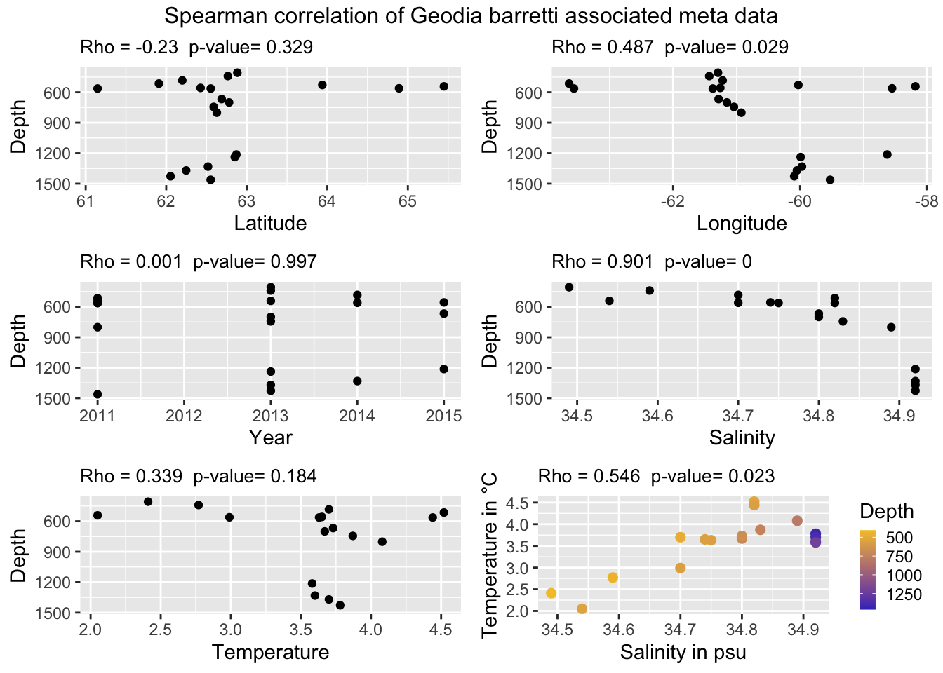
Figure 1.8: Correlation of depth with other environmental parameters/predictor variables across samples of G. barretti.
library(usdm)
md$Species <- NULL
md$unified_ID <- NULL
vif1 <- vif(md)
vif1$VIF <- round(vif1$VIF, digits = 2)

md$MeanBotSalinity_PSU <- NULL
md$MeanBottomTemp_Cdeg <- NULL
vif2 <- vif(md)
vif2$VIF <- round(vif2$VIF, digits = 2)

library(dplyr)
vifs <- full_join(vif1, vif2, by = c(Variables = "Variables"))
colnames(vifs) <- c("Variables", "All predictors", "Subset")
vifs[c(5, 6), 3] <- ""

library(kableExtra)
options(kableExtra.html.bsTable = T)

cap <- paste("VIF for extensive and simplified models for", text_spec("G. barretti", italic = T))

kable(vifs, longtable = T, booktabs = T, caption = cap, row.names = F) %>% kable_styling(bootstrap_options = c("striped", "hover", "bordered", "condensed", "responsive"),
full_width = F, latex_options = c("striped", "scale_down"))| Variables | All predictors | Subset |
|---|---|---|
| Depth | 22.15 | 5.91 |
| Latitude | 11.63 | 10.31 |
| Longitude | 16.59 | 13.38 |
| YEAR | 1.73 | 1.46 |
| MeanBotSalinity_PSU | 61.13 | |
| MeanBottomTemp_Cdeg | 47.52 |
With this subset, the collinearity becomes even more pronounced. Salinity, temperature and depth are strongly correlated and the VIFs indicated that they should not be included in a model together. This correlation is partly due to physical properties of water. Density of water increases with increasing salinity and decreasing temperature. To a lesser extent, longitude and lattitude are collinear in our sampling. However, removing the predictor variables salinity and temperature mititgated/lowered the effect of collinearity.