4 Inter-omics

The inter-omics analyses are comprised of three parts. In the first part, we evaluate congruency of the prokaryotic and metabolomic data set as a whole using numerical methods (Mantel test) and ordination (Procrustes rotation and Protest). The second part consists of generating a microbial interaction network and annotating it with depth response of the OTUs and correlation with the barettin signal. In the third part, we rank OTUs based on properties hypothesised to be true for the producer of barettin.

4.1 Mantel test and procrustes rotations

4.1.1 Libraries and functions

4.1.2 Data sets

# LOAD DATA
micro <- read.csv("data/OTU_all_R.csv", header = T, sep = ";")
colnames(micro)[colnames(micro) == "Sample_ID"] <- "unified_ID"
micro <- micro[order(micro$unified_ID), ]
rownames(micro) <- micro$unified_ID
micro["spec"] <- str_sub(micro$unified_ID, 1, 2)

meta_data <- read.csv("data/PANGAEA_Final.csv", header = T, sep = ";")
masslynx <- meta_data
masslynx <- masslynx[c("unified_ID", "LC.MS.HILIC.positive", "LC.MS.HILIC.negative", "LC.MS.RP.positive", "LC.MS.RP.negative")]
colnames(masslynx) <- c("unified_ID", "H_p", "H_n", "R_p", "R_n")
masslynx <- na.omit(masslynx)
masslynx["HILIC_pos"] <- str_sub(masslynx$H_p, 1, -3)
masslynx["HILIC_neg"] <- str_sub(masslynx$H_n, 1, -3)
masslynx["RP_pos"] <- str_sub(masslynx$R_p, 1, -3)
masslynx["RP_neg"] <- str_sub(masslynx$R_n, 1, -3)

# load one set of experiments at a time, i.e. CLEANED, ION or PC_GROUPS

### CLEANED
hilic_pos <- read.csv("data/HILIC_pos_20190417_cleaned.csv", header = T, sep = ",")
hilic_neg <- read.csv("data/HILIC_neg_20190421_cleaned.csv", header = T, sep = ",")
rp_pos <- read.csv("data/RP_pos_20190421_cleaned.csv", header = T, sep = ",")
rp_neg <- read.csv("data/RP_neg_20190422_cleaned.csv", header = T, sep = ",")

### ION
hilic_pos <- read.csv("data/HILIC_pos_20190417_cleaned_MH.csv", header = T, sep = ",")
hilic_neg <- read.csv("data/HILIC_neg_20190421_cleaned_MH.csv", header = T, sep = ",")
rp_pos <- read.csv("data/RP_pos_20190421_cleaned_MH.csv", header = T, sep = ",")
rp_neg <- read.csv("data/RP_neg_20190422_cleaned_MH.csv", header = T, sep = ",")

### PC_GROUPS
hilic_pos <- read.csv("data/HILIC_pos_20190417_cleaned_pcgroup.csv", header = T, sep = ",")
hilic_neg <- read.csv("data/HILIC_neg_20190421_cleaned_pcgroup.csv", header = T, sep = ",")
rp_pos <- read.csv("data/RP_pos_20190421_cleaned_pcgroup.csv", header = T, sep = ",")
rp_neg <- read.csv("data/RP_neg_20190422_cleaned_pcgroup.csv", header = T, sep = ",")

4.1.3 Mantel test code and tabular output

### =============================== MANTEL TEST=================================

# run one of this at a time
metabolomes <- gymnastics(hilic_pos, "H_p")
metabolomes <- gymnastics(hilic_neg, "H_n")
metabolomes <- gymnastics(rp_pos, "R_p")
metabolomes <- gymnastics(rp_neg, "R_n")

# run this
congruent_dfs <- congruency(metabolomes)

# run one of these: MANTEL TEST
diagnostics_hp_cleaned <- cloak(congruent_dfs = congruent_dfs, experiment = "HILIC pos", filtering = "cleaned")
diagnostics_hn_cleaned <- cloak(congruent_dfs = congruent_dfs, experiment = "HILIC neg", filtering = "cleaned")
diagnostics_rp_cleaned <- cloak(congruent_dfs = congruent_dfs, experiment = "RP pos", filtering = "cleaned")
diagnostics_rn_cleaned <- cloak(congruent_dfs = congruent_dfs, experiment = "RP neg", filtering = "cleaned")

diagnostics_hp_ion <- cloak(congruent_dfs = congruent_dfs, experiment = "HILIC pos", filtering = "ion")
diagnostics_hn_ion <- cloak(congruent_dfs = congruent_dfs, experiment = "HILIC neg", filtering = "ion")
diagnostics_rp_ion <- cloak(congruent_dfs = congruent_dfs, experiment = "RP pos", filtering = "ion")
diagnostics_rn_ion <- cloak(congruent_dfs = congruent_dfs, experiment = "RP neg", filtering = "ion")

diagnostics_hp_pc_group <- cloak(congruent_dfs = congruent_dfs, experiment = "HILIC pos", filtering = "pc_group")
diagnostics_hn_pc_group <- cloak(congruent_dfs = congruent_dfs, experiment = "HILIC neg", filtering = "pc_group")
diagnostics_rp_pc_group <- cloak(congruent_dfs = congruent_dfs, experiment = "RP pos", filtering = "pc_group")
diagnostics_rn_pc_group <- cloak(congruent_dfs = congruent_dfs, experiment = "RP neg", filtering = "pc_group")


### Combine all test results into one file

diagnostics <- diagnostics_hp_cleaned
diagnostics <- rbind(diagnostics, diagnostics_hn_cleaned, diagnostics_rp_cleaned, diagnostics_rn_cleaned, diagnostics_hp_pc_group, diagnostics_hn_pc_group, diagnostics_rp_pc_group, 
    diagnostics_rn_pc_group, diagnostics_hp_ion, diagnostics_hn_ion, diagnostics_rp_ion, diagnostics_rn_ion)
diagnostics
write.csv(diagnostics, "mantel_stats_FUN.csv")

diagnostics <- read.csv("data/mantel_stats_FUN.csv")
diagnostics$X <- NULL
diagnostics <- diagnostics[, c("statistic", "signif", "micro_samples", "micro_OTUs", "meta_samples", "meta_features", "Sponge.species", "Experiment", "data.set")]

options(kableExtra.html.bsTable = T)
kable(diagnostics, col.names = c("Mantel statistic r", "significance", "N microbiome samples", "N OTUs", "N metabolome samples", "N features", "Sponge species", 
    "Experiment", "data set"), longtable = T, booktabs = T, caption = "Mantel test diagnostics diagnositcs comparing the microbiome and metabolome of the same sponge specimens", 
    row.names = FALSE) %>% add_header_above(c(Diagnostics = 6, `Data set attribution` = 3)) %>% kable_styling(bootstrap_options = c("striped", "hover", "bordered", 
    "condensed", "responsive"), font_size = 12, full_width = F, latex_options = c("striped", "scale_down"))

Mantel statistic r	significance	N microbiome samples	N OTUs	N metabolome samples	N features	Sponge species	Experiment	data set
0.6076416	0.004	10	420	10	3507	Geodia barretti	HILIC pos	cleaned
0.3857788	0.011	13	461	13	3507	Stryphnus fortis	HILIC pos	cleaned
0.4576405	0.008	15	135	15	3507	Weberella bursa	HILIC pos	cleaned
0.4516469	0.006	10	420	10	2808	Geodia barretti	HILIC neg	cleaned
0.1513297	0.186	13	461	13	2808	Stryphnus fortis	HILIC neg	cleaned
0.1854966	0.168	15	135	15	2808	Weberella bursa	HILIC neg	cleaned
-0.2014493	0.833	10	420	10	4673	Geodia barretti	RP pos	cleaned
0.3127632	0.064	13	461	13	4673	Stryphnus fortis	RP pos	cleaned
0.3323657	0.035	15	135	15	4673	Weberella bursa	RP pos	cleaned
-0.2465894	0.845	9	420	9	3166	Geodia barretti	RP neg	cleaned
0.1960950	0.173	13	461	13	3166	Stryphnus fortis	RP neg	cleaned
0.1721750	0.174	15	135	15	3166	Weberella bursa	RP neg	cleaned
0.5836627	0.009	10	420	10	2212	Geodia barretti	HILIC pos	pc_group
0.4082626	0.016	13	461	13	2212	Stryphnus fortis	HILIC pos	pc_group
0.4483931	0.012	15	135	15	2212	Weberella bursa	HILIC pos	pc_group
0.3951252	0.018	10	420	10	1351	Geodia barretti	HILIC neg	pc_group
0.3211093	0.040	13	461	13	1351	Stryphnus fortis	HILIC neg	pc_group
0.0315675	0.414	15	135	15	1351	Weberella bursa	HILIC neg	pc_group
-0.1600791	0.774	10	420	10	2736	Geodia barretti	RP pos	pc_group
0.3181249	0.064	13	461	13	2736	Stryphnus fortis	RP pos	pc_group
0.3008501	0.067	15	135	15	2736	Weberella bursa	RP pos	pc_group
-0.1879022	0.790	9	420	9	1678	Geodia barretti	RP neg	pc_group
0.2034548	0.156	13	461	13	1678	Stryphnus fortis	RP neg	pc_group
0.1507257	0.198	15	135	15	1678	Weberella bursa	RP neg	pc_group
0.3351779	0.050	10	420	10	105	Geodia barretti	HILIC pos	ion
0.2908357	0.086	13	461	13	105	Stryphnus fortis	HILIC pos	ion
0.4683599	0.010	15	135	15	105	Weberella bursa	HILIC pos	ion
0.4429513	0.005	10	420	10	123	Geodia barretti	HILIC neg	ion
0.0727247	0.320	13	461	13	123	Stryphnus fortis	HILIC neg	ion
0.2320236	0.115	15	135	15	123	Weberella bursa	HILIC neg	ion
-0.2569170	0.908	10	420	10	171	Geodia barretti	RP pos	ion
0.3070980	0.083	13	461	13	171	Stryphnus fortis	RP pos	ion
0.2656853	0.072	15	135	15	171	Weberella bursa	RP pos	ion
-0.1220077	0.703	9	420	9	105	Geodia barretti	RP neg	ion
-0.0505950	0.597	13	461	13	105	Stryphnus fortis	RP neg	ion
0.1218225	0.217	15	135	15	105	Weberella bursa	RP neg	ion

dig <- diagnostics[diagnostics$signif <= 0.05, ]
a <- aggregate(dig, by = list(dig$Sponge.species, dig$Experiment, dig$data.set), FUN = "length")
summary(a$Group.1)

##  Geodia barretti Stryphnus fortis  Weberella bursa 
##                6                3                4

summary(a$Group.2)

## HILIC neg HILIC pos    RP neg    RP pos 
##         4         8         0         1

summary(a$Group.3)

##  cleaned      ion pc_group 
##        5        3        5

rm(diagnostics_hp_cleaned, diagnostics_hn_cleaned, diagnostics_rp_cleaned, diagnostics_rn_cleaned, diagnostics_hp_ion, diagnostics_hn_ion, diagnostics_rp_ion, 
    diagnostics_rn_ion, diagnostics_hp_pc_group, diagnostics_hn_pc_group, diagnostics_rp_pc_group, diagnostics_rn_pc_group)
rm(hilic_pos, hilic_neg, rp_pos, rp_neg)

As we can see from the table, in 13 cases, the Mantel test returns a significant correlation between the two matrices. Above you can see the the significant tests broken down by sponge species, HPCL-experiment and filtering approach.

4.1.4 Procrustes rotation and protest code and tabular output

### =============================== PROTEST ====================================

# run one of this at a time
metabolomes <- gymnastics(hilic_pos, "H_p")
metabolomes <- gymnastics(hilic_neg, "H_n")
metabolomes <- gymnastics(rp_pos, "R_p")
metabolomes <- gymnastics(rp_neg, "R_n")

# run this
congruent_dfs <- congruency(metabolomes)

# run one of these: PROTEST TEST
diagnostics_hp_cleaned <- ordination(congruent_dfs = congruent_dfs, experiment = "HILIC pos", filtering = "cleaned")
diagnostics_hn_cleaned <- ordination(congruent_dfs = congruent_dfs, experiment = "HILIC neg", filtering = "cleaned")
diagnostics_rp_cleaned <- ordination(congruent_dfs = congruent_dfs, experiment = "RP pos", filtering = "cleaned")
diagnostics_rn_cleaned <- ordination(congruent_dfs = congruent_dfs, experiment = "RP neg", filtering = "cleaned")

diagnostics_hp_ion <- ordination(congruent_dfs = congruent_dfs, experiment = "HILIC pos", filtering = "ion")
diagnostics_hn_ion <- ordination(congruent_dfs = congruent_dfs, experiment = "HILIC neg", filtering = "ion")
diagnostics_rp_ion <- ordination(congruent_dfs = congruent_dfs, experiment = "RP pos", filtering = "ion")
diagnostics_rn_ion <- ordination(congruent_dfs = congruent_dfs, experiment = "RP neg", filtering = "ion")

diagnostics_hp_pc_group <- ordination(congruent_dfs = congruent_dfs, experiment = "HILIC pos", filtering = "pc_group")
diagnostics_hn_pc_group <- ordination(congruent_dfs = congruent_dfs, experiment = "HILIC neg", filtering = "pc_group")
diagnostics_rp_pc_group <- ordination(congruent_dfs = congruent_dfs, experiment = "RP pos", filtering = "pc_group")
diagnostics_rn_pc_group <- ordination(congruent_dfs = congruent_dfs, experiment = "RP neg", filtering = "pc_group")


### Combine all test results into one file

diagnostics <- diagnostics_hp_cleaned
diagnostics <- rbind(diagnostics, diagnostics_hn_cleaned, diagnostics_rp_cleaned, diagnostics_rn_cleaned, diagnostics_hp_pc_group, diagnostics_hn_pc_group, diagnostics_rp_pc_group, 
    diagnostics_rn_pc_group, diagnostics_hp_ion, diagnostics_hn_ion, diagnostics_rp_ion, diagnostics_rn_ion)
diagnostics

write.csv(diagnostics, "protest_stats_FUN.csv")

rm(diagnostics_hp_cleaned, diagnostics_hn_cleaned, diagnostics_rp_cleaned, diagnostics_rn_cleaned, diagnostics_hp_ion, diagnostics_hn_ion, diagnostics_rp_ion, 
    diagnostics_rn_ion, diagnostics_hp_pc_group, diagnostics_hn_pc_group, diagnostics_rp_pc_group, diagnostics_rn_pc_group, diagnostics)
rm(hilic_pos, hilic_neg, rp_pos, rp_neg)

diagnostics <- read.csv("data/protest_stats_FUN.csv")
diagnostics$X <- NULL
diagnostics <- diagnostics[, c("Procrustes.SS", "correlation.in.sym..rotation", "signif", "micro_samples", "micro_OTUs", "meta_samples", "meta_features", "Sponge.species", 
    "Experiment", "data.set")]

options(kableExtra.html.bsTable = T)
kable(diagnostics, col.names = c("Procrustes sum of squares", "correlation in symmetric rotation", "significance", "N microbiome samples", "N OTUs", "N metabolome samples", 
    "N features", "Sponge species", "Experiment", "data set"), longtable = T, booktabs = T, caption = "Protest diagnostics comparing the microbiome and metabolome of the same sponge specimens", 
    row.names = FALSE) %>% add_header_above(c(Diagnostics = 7, `Data set attribution` = 3)) %>% kable_styling(bootstrap_options = c("striped", "hover", "bordered", 
    "condensed", "responsive"), font_size = 12, full_width = F, latex_options = c("striped", "scale_down"))

Procrustes sum of squares	correlation in symmetric rotation	significance	N microbiome samples	N OTUs	N metabolome samples	N features	Sponge species	Experiment	data set
0.4901473	0.7140397	0.009	10	420	10	3507	Geodia barretti	HILIC pos	cleaned
0.3360196	0.8148499	0.001	13	461	13	3507	Stryphnus fortis	HILIC pos	cleaned
0.6451196	0.5957184	0.009	15	135	15	3507	Weberella bursa	HILIC pos	cleaned
0.5056719	0.7030847	0.015	10	420	10	2808	Geodia barretti	HILIC neg	cleaned
0.7144829	0.5343380	0.043	13	461	13	2808	Stryphnus fortis	HILIC neg	cleaned
0.6454847	0.5954119	0.003	15	135	15	2808	Weberella bursa	HILIC neg	cleaned
0.7241690	0.5251961	0.124	10	420	10	4673	Geodia barretti	RP pos	cleaned
0.5535784	0.6681479	0.005	13	461	13	4673	Stryphnus fortis	RP pos	cleaned
0.9089831	0.3016901	0.513	15	135	15	4673	Weberella bursa	RP pos	cleaned
0.7744081	0.4749652	0.229	9	420	9	3166	Geodia barretti	RP neg	cleaned
0.7769037	0.4723307	0.107	13	461	13	3166	Stryphnus fortis	RP neg	cleaned
0.9426954	0.2393838	0.656	15	135	15	3166	Weberella bursa	RP neg	cleaned
0.4903060	0.7139285	0.008	10	420	10	2212	Geodia barretti	HILIC pos	pc_group
0.6122646	0.6226840	0.009	13	461	13	2212	Stryphnus fortis	HILIC pos	pc_group
0.5611609	0.6624494	0.002	15	135	15	2212	Weberella bursa	HILIC pos	pc_group
0.4442919	0.7454583	0.007	10	420	10	1351	Geodia barretti	HILIC neg	pc_group
0.6072203	0.6267214	0.013	13	461	13	1351	Stryphnus fortis	HILIC neg	pc_group
0.7647882	0.4849864	0.062	15	135	15	1351	Weberella bursa	HILIC neg	pc_group
0.7332277	0.5165001	0.146	10	420	10	2736	Geodia barretti	RP pos	pc_group
0.5557670	0.6665081	0.002	13	461	13	2736	Stryphnus fortis	RP pos	pc_group
0.9184545	0.2855616	0.579	15	135	15	2736	Weberella bursa	RP pos	pc_group
0.7952845	0.4524550	0.314	9	420	9	1678	Geodia barretti	RP neg	pc_group
0.7513407	0.4986575	0.089	13	461	13	1678	Stryphnus fortis	RP neg	pc_group
0.9669093	0.1819085	0.851	15	135	15	1678	Weberella bursa	RP neg	pc_group
0.7744285	0.4749437	0.254	9	420	9	3166	Geodia barretti	HILIC pos	ion
0.7768298	0.4724090	0.119	13	461	13	3166	Stryphnus fortis	HILIC pos	ion
0.9427350	0.2393010	0.671	15	135	15	3166	Weberella bursa	HILIC pos	ion
0.3977778	0.7760297	0.005	10	420	10	123	Geodia barretti	HILIC neg	ion
0.7620196	0.4878323	0.101	13	461	13	123	Stryphnus fortis	HILIC neg	ion
0.6263664	0.6112558	0.007	15	135	15	123	Weberella bursa	HILIC neg	ion
0.6879735	0.5585933	0.083	10	420	10	171	Geodia barretti	RP pos	ion
0.6735153	0.5713884	0.038	13	461	13	171	Stryphnus fortis	RP pos	ion
0.9830213	0.1303022	0.961	15	135	15	171	Weberella bursa	RP pos	ion
0.7788793	0.4702347	0.271	9	420	9	105	Geodia barretti	RP neg	ion
0.9754054	0.1568265	0.767	13	461	13	105	Stryphnus fortis	RP neg	ion
0.9595716	0.2010681	0.791	15	135	15	105	Weberella bursa	RP neg	ion

dig <- diagnostics[diagnostics$signif <= 0.05, ]
a <- aggregate(dig, by = list(dig$Sponge.species, dig$Experiment, dig$data.set), FUN = "length")
summary(a$Group.1)

##  Geodia barretti Stryphnus fortis  Weberella bursa 
##                5                7                4

summary(a$Group.2)

## HILIC neg HILIC pos    RP neg    RP pos 
##         7         6         0         3

summary(a$Group.3)

##  cleaned      ion pc_group 
##        7        3        6

Out of the 36 tests performed, 16 are significant (p \(\leq\) 0.05). Immediately above you can see the the significant tests broken down by sponge species, HPCL-experiment and filtering approach.

4.2 Correlating barettin and prokaryotic relative abundance

cmp <- read.csv("data/metabolite_master_20190605.csv", header = T, sep = ",")
cmp$X <- NULL
meta_data <- read.csv("data/Steffen_et_al_metadata_PANGAEA.csv", header = T, sep = ";")
micro <- read.csv("data/OTU_all_R.csv", header = T, sep = ";")

# preparing meta data
meta_data_prep <- function(meta_data) {
    meta_data <- meta_data[, c("unified_ID", "Depth", "Latitude", "Longitude", "MeanBottomTemp_Cdeg", "MeanBotSalinity_PSU", "YEAR")]
    colnames(meta_data) <- c("unified_ID", "Depth", "Latitude", "Longitude", "Temperature", "Salinity", "Year")
    meta_data <- meta_data[!(str_sub(meta_data$unified_ID, 1, 2) == "QC"), ]
    meta_data[] <- lapply(meta_data, function(x) if (is.factor(x)) 
        factor(x) else x)
    # Gb12, Gb20 and Gb21 are missing temperature and salinity. Imputing data from closeby samples:
    meta_data$Salinity[meta_data$unified_ID == "Gb12"] <- 34.92
    meta_data$Salinity[meta_data$unified_ID == "Gb20"] <- 34.92
    meta_data$Salinity[meta_data$unified_ID == "Gb21"] <- 34.56
    meta_data$Temperature[meta_data$unified_ID == "Gb12"] <- 3.71
    meta_data$Temperature[meta_data$unified_ID == "Gb20"] <- 3.65
    meta_data$Temperature[meta_data$unified_ID == "Gb21"] <- 2.32
    meta_data["spec"] <- str_sub(meta_data$unified_ID, 1, 2)
    meta_data <- meta_data[order(meta_data$unified_ID), ]
    return(meta_data)
}

meta_data <- meta_data_prep(meta_data)

# separating OTU tables by sponge
OTU_prep_sqrt <- function(micro) {
    rownames(micro) <- micro$Sample_ID
    micro$Sample_ID <- NULL
    # micro <- sqrt(micro) #sqrt could be toggled on/off here
    
    micro_gb <- micro[(str_sub(rownames(micro), 1, 2) == "Gb"), ]
    micro_sf <- micro[(str_sub(rownames(micro), 1, 2) == "Sf"), ]
    micro_wb <- micro[(str_sub(rownames(micro), 1, 2) == "Wb"), ]
    
    micro_gb <- micro_gb[, colSums(micro_gb != 0) > 0]
    micro_sf <- micro_sf[, colSums(micro_sf != 0) > 0]
    micro_wb <- micro_wb[, colSums(micro_wb != 0) > 0]
    micros <- list(gb = micro_gb, sf = micro_sf, wb = micro_wb)
    return(micros)
}

micro_ds <- OTU_prep_sqrt(micro)

# calculating overall relative abundance of each OTU per sample
overall_rabdc <- function(micros) {
    mic <- micros
    n <- 0
    k <- dim(mic)[1]
    mic["rowsum"] <- apply(mic, 1, sum)
    
    while (n < k) {
        n <- n + 1
        mic[n, ] <- mic[n, ]/(mic$rowsum[n])
    }
    
    mic$rowsum <- NULL
    mic <- data.frame(t(mic))
    # mic['avg_rel_abdc'] <- apply(mic, 1, mean) mic['occurrence'] <- ifelse(mic$avg>0.0025, 'common', 'rare')
    return(mic)
}

rabdc <- lapply(micro_ds, overall_rabdc)

# preparing congruent data sets
common_samples <- intersect(colnames(rabdc$gb), cmp$unified_ID)
rabdc <- rabdc$gb[, colnames(rabdc$gb) %in% common_samples]
rabdc <- data.frame(t(rabdc))

cmp <- cmp[cmp$unified_ID %in% common_samples, ]
cmp[] <- lapply(cmp, function(x) if (is.factor(x)) factor(x) else x)
cmp <- cmp[order((cmp$unified_ID)), ]

# all(rownames(rabdc)==cmp$unified_ID)

# CORRELATION for Gb and Sf

bar_cor <- function(rabdc_df, cmp) {
    barettin <- data.frame(colnames(rabdc_df))
    colnames(barettin) <- "XOTU"
    barettin["barettin_estimate_P"] <- NA
    barettin["barettin_p_val_P"] <- NA
    barettin["barettin_estimate_S"] <- NA
    barettin["barettin_p_val_S"] <- NA
    
    n <- 0
    k <- dim(barettin)[1]
    while (n < k) {
        n <- n + 1
        barettin$barettin_estimate_P[n] <- cor.test(as.numeric(rabdc_df[, n]), cmp$bar, method = "pearson")$estimate
        barettin$barettin_p_val_P[n] <- cor.test(as.numeric(rabdc_df[, n]), cmp$bar, method = "pearson")$p.value
        barettin$barettin_estimate_S[n] <- cor.test(as.numeric(rabdc_df[, n]), cmp$bar, method = "spearman")$estimate
        barettin$barettin_p_val_S[n] <- cor.test(as.numeric(rabdc_df[, n]), cmp$bar, method = "spearman")$p.value
    }
    
    barettin["barettin_fdr_P"] <- NA
    barettin["barettin_fdr_S"] <- NA
    barettin$barettin_fdr_P <- p.adjust(barettin$barettin_p_val_P, method = "fdr")
    barettin$barettin_fdr_S <- p.adjust(barettin$barettin_p_val_S, method = "fdr")
    return(barettin)
}

barettin_cor <- bar_cor(rabdc, cmp)

# write.csv(barettin_cor, 'data/GB_OTU_barettin_correlation.csv', row.names = F)

par(mfrow = c(1, 3))
hist(barettin_cor$barettin_estimate_P, main = "Pearson's pmcc: \n OTU rel abdc ~ barettin signal", xlab = "Product moment \n correlation coefficient")
hist(barettin_cor$barettin_p_val_P, breaks = 20, main = "Pearson's pmcc p-value", xlab = "p-value")
hist(barettin_cor$barettin_fdr_P, breaks = 20, main = "Pearson's pmcc \n fdr corrected p-value", xlab = "FDR corrected p-value")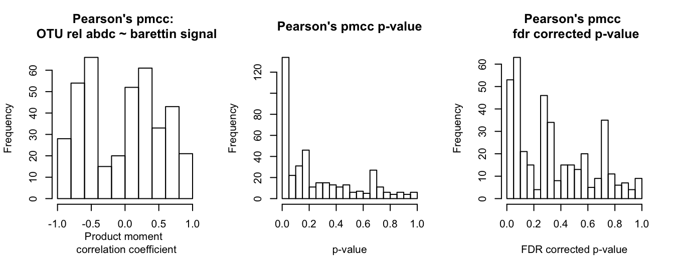

par(mfrow = c(1, 1))

par(mfrow = c(1, 3))
hist(barettin_cor$barettin_estimate_S, main = "Spearman's rho: \n OTU rel abdc ~ barettin signal", xlab = "Rho")
hist(barettin_cor$barettin_p_val_S, breaks = 20, main = "Spearman's rho p-value", xlab = "p-value")
hist(barettin_cor$barettin_fdr_S, breaks = 20, main = "Spearman's rho \n fdr corrected p-value", xlab = "FDR corrected p-value")

par(mfrow = c(1, 1))

# For Sf, for shortlist
cmp <- read.csv("data/metabolite_master_20190605.csv", header = T, sep = ",")
cmp$X <- NULL
rabdc <- lapply(micro_ds, overall_rabdc)
common_samples <- intersect(colnames(rabdc$sf), cmp$unified_ID)
rabdc <- rabdc$sf[, colnames(rabdc$sf) %in% common_samples]
rabdc <- data.frame(t(rabdc))

cmp <- cmp[cmp$unified_ID %in% common_samples, ]
cmp[] <- lapply(cmp, function(x) if (is.factor(x)) factor(x) else x)
cmp <- cmp[order((cmp$unified_ID)), ]
all(rownames(rabdc) == cmp$unified_ID)

## [1] TRUE

barettin_cor <- bar_cor(rabdc, cmp)
# write.csv(barettin_cor, 'data/SF_OTU_barettin_correlation.csv', row.names = F)

4.3 Microbial interaction network

4.3.1 Generating network based on different algorithms

The overall goal of the subsequent seqctions of code is to produce a microbial interation network for Geodia barretti. Nodes will be OTUs/ASVs from Geodia barretti samples and edges represent an interaction between those OTUs/ASVs. In this first part, we will employ different algorithms for network building. Network building algorithms are mannifold and their results not uncontroversial, thus the recommended strategy is to use different methods and merge the resulting networks to one consensus representation (Weiss et al., 2016), which we will do in the second part.

The original data set from 14 specimens of Geodia barretti contained 420 OTUs/ASVs. To reduce sparsity, we removed OTUs/ASVs with two or less non-zero values resulting in a data set containing 289 OTUs/ASVs. This data set was used for network inference with the following methods:

MENA Pipeline
fastLSA
SparCC
Maximal information coefficient MIC

4.3.1.1 Molecular Ecological Network Analysis (MENA) Pipeline

The implementation of MENA (Deng et al., 2012; Zhou, Deng et al., 2010; Zhou, Deng et al.,2011) can be accessed at http://ieg4.rccc.ou.edu/mena. The data set was saved as tab separated values and all zeros were converted to blanks. No further filtering for non-zero values was done (more than two non-zero values). For data preparation, default settings were applied, i.e. missing data was only filled with 0.01 in blanks with paired valid values, logarithm was taken, Pearson correlation coefficient was selected. Likewise, Random matrix theory settings were kept at defaults, decreasing the cutoff from the top using Regress Poisson distribution only. The cutoff of 0.800 was chosen for the similarity matrix to construct the network, corresponding to a Chi-square test on Poisson distribution of 99.191 and a p-value of 0.001. This resulted in a network with 241 nodes and 3582 edges.

A second analysis was produced with the same settings except building the similarity matrix based on Spearman’s Rho. The cutoff of 0.820 was chosen for the similarity matrix to construct the network, corresponding to a Chi-square test on Poisson distribution of 98.417 and a p-value of 0.001. This resulted in a network with 252 nodes and 2216 edges.

Network properties and parameters are summarized in MENA_network_parameters_Feb2019.xlsx.

4.3.1.2 Local Similarity Analysis: fastLSA

The command line program for calcularing local similarity (Durno et al., 2013) was downloaded from http://hallam.microbiology.ubc.ca/fastLSA/install/index.html and run specifying the input file, no time lag (-d 0) and significance level alpha (-a 0.05). All other paramters were kept at their default values. The input data set was a tab delimited text file stripped of OTU labels or sample IDs.

$ ./fastLSA -i ../gb_289_feb2019.txt -d 0 -a 0.05 -o ../gb_289_feb2019.out

The output file, as specified on the website, containes five columns. ‘index1’ and ‘index2’ represent the significant paired indices ranging from 0 to n-1 (OTUs/ASVs). LSA denotes the LSA statistic of each pair, lag was set to 0 with the -d flag and the p-valueBound column provides the p-value’s upper boundary for the significantly paired p-value.

To produce comparable data sets, we replaced the indices with their OTU IDs and removed superfluous columns.

fastLSA <- read.csv("data/gb_289_feb2019.out", header = T, sep = "")
key <- read.csv("data/fastLSA_index_otu_CORRECTEDfeb2019.csv", header = T, sep = ";")

fastLSA$index1_otu <- key$fastLSA_OTU[match(fastLSA$index1, key$fastLSA_index)]
fastLSA$index2_otu <- key$fastLSA_OTU[match(fastLSA$index2, key$fastLSA_index)]

fastLSA$index1 <- NULL
fastLSA$index2 <- NULL
fastLSA$lag <- NULL
fastLSA$X <- NULL
fastLSA <- fastLSA[, c(3, 4, 1, 2)]
fastLSA <- fastLSA[order(fastLSA$p.valueBound), ]

# write.csv(fastLSA, 'fastLSA_for_networks.csv')
rm(key)

LSA scores range from -1 for strong negatively correlations to 1, for strong positive correlations. There were no negative correlations in this data setand we refrained from scaleding the LSA score furhter. The resulting network contrained 129 nodes and 207 edges.

4.3.1.3 SparCC

SparCC (Friedman and Alm, 2012) is a network building algorithm for compositional data and can be found at https://bitbucket.org/yonatanf/sparcc.

Prior to running it I had to get help as there was a minor issue during compilation. SparCC needed specific versions of numpy, panda and python to run properly, which is easiest accomodated in a specific environment. The OTU table needs to be windows formatted text. The embedded code is an example, for the analysis, 500 iterations were combined.

$ cd to working directory with SparCC and the data set gb_289.csv
$ source activate sparcc
python SparCC.py ../gb_sparcc.txt -c ../gb_sparcc_cor_file.txt -v 
../gb_sparcc_coverage_file.txt -i 5
$ deactivate

Create a results directory and redirect all the output there. Pseudo p-value Calculation, generates -n shuffled data sets:

$ mkdir results #creates output directory
$ python MakeBootstraps.py ../gb_sparcc.txt -n 5 -t permutation_#.txt -p ../results/

And run SparCC.py on all the re-shuffled data sets:

$ python SparCC.py ../results/permutation_0.txt -i 5 --cor_file=../results/perm_cor_0.txt
$ python SparCC.py ../results/permutation_1.txt -i 5 --cor_file=../results/perm_cor_1.txt
$ python SparCC.py ../results/permutation_2.txt -i 5 --cor_file=../results/perm_cor_2.txt
$ python SparCC.py ../results/permutation_3.txt -i 5 --cor_file=../results/perm_cor_3.txt
$ python SparCC.py ../results/permutation_4.txt -i 5 --cor_file=../results/perm_cor_4.txt

Generate p-values:

$ python PseudoPvals.py ../results/gb_sparcc_cor_file.txt ../results/perm_cor_#.txt 5 
-o ../results/pvals.two_sided.txt -t two_sided

Formatting the resulting data set like so:

library(reshape2)
cor_file <- read.csv("data/gb_sparcc_cor_file_289.csv", header = T, sep = ";")
p_vals <- read.csv("data/gb_289_pvals.two_sided.csv", header = T, sep = ";")

# make OTU ID the rowname
rownames(cor_file) <- cor_file[, 1]
cor_file[, 1] <- NULL
rownames(p_vals) <- p_vals[, 1]
p_vals[, 1] <- NULL
# check ds congruency
all(colnames(cor_file) == rownames(cor_file))
all(colnames(p_vals) == rownames(p_vals))

# melt into long format, all vs all comparison: 289^2=83521 rows
cor_file_m <- melt(as.matrix(cor_file))
p_vals_m <- melt(as.matrix(p_vals))

all(cor_file_m$Var1 == p_vals_m$Var1)
all(cor_file_m$Var2 == p_vals_m$Var2)

# complete data set with p_vals and 'correlation coeff'
cor_file_m["p_vals"] <- p_vals_m$value

# This removes AB - BA duplicates but still contains self comprisons, AA, BB,CC etc.
cols <- c("Var1", "Var2")
newdf <- cor_file_m[, cols]  #generate new data set with just those two
# a <- Sys.time()
for (i in 1:nrow(cor_file_m)) {
    newdf[i, ] = sort(cor_file_m[i, cols])
}
# b <- Sys.time() b-a

cor_file_shortened <- cor_file_m[!duplicated(newdf), ]  #and can be removed with duplicate
cor_file_shortened <- cor_file_shortened[which(cor_file_shortened$Var1 != cor_file_shortened$Var2), ]  # removing self comparison
colnames(cor_file_shortened) <- c("Var1_SparCC", "Var2_SparCC", "SparCC", "pSparCC")  #41616
write.csv(cor_file_shortened, "data/SparCC_for_networks.csv")
rm(cor_file_m, newdf, p_vals_m, i, cols)

4.3.1.4 Maximal information coefficient MIC

MIC for pairwise interaction was calculated with the R package minearva. The MIC is part of a statistic called Maximal Information-Based Nonparametric Exploration (MINE).

library(minerva)

OTU <- read.csv("data/gb_289.csv", header = T, sep = ";")
rownames(OTU) <- OTU[, 1]
OTU[, 1] <- NULL
OTU <- as.data.frame(t(OTU))

# Calculate MIC of original data set.
MINE <- mine(OTU)
MIC <- MINE$MIC  #dim(MIC): 289 289

Obtaining p-values for this statistic can be achieved by permutation of the original OTU table as below or empirically, by selecting the thousand strongest interactions.

# 10 needs to be replaced with 1000 for final version, three times!!!  reshuffling the OTU table, saving the MIC to a list, a total of 1000 times
n <- 0
results <- list()

# For reproducibility, one could e.g.: set.seed(1984)

# c <- Sys.time()
while (n < 1000) {
    n <- n + 1
    mock <- apply(OTU, MARGIN = 2, sample)
    mock_mine <- mine(mock)
    results[[n]] <- mock_mine$MIC
}
# d <- Sys.time() d-c

# for every element of the true matrix, go through all the same elements in the 1000 generated mock matrix MIC indices and count how many of those are
# greater.
MIC <- MINE$MIC

e_values <- matrix(nrow = nrow(MIC), ncol = ncol(MIC), data = 0)
for (i in 1:nrow(MIC)) {
    for (j in 1:ncol(MIC)) {
        n <- 0
        while (n < 1000) {
            n <- n + 1
            if (results[[n]][i, j] >= MIC[i, j]) {
                e_values[i, j] <- e_values[i, j] + 1
            }
        }
    }
}

e_values <- e_values/1000
# write.csv(e_values, 'data/MIC_e_values.csv')

For n=1000, the first part takes about 8 mins on one core, the second part about 2 min. The relevant output is saved in the initial calculations of the MIC and the corresponding e-values are in e_values. These are symmetric matrices that will be reduced to a long table with unique OTUs/ASVs pairs, their MIC and the e-value. For clarity, all other files are removed.

rm(MINE, mock, mock_mine, results)

# transforming symmetric matrix to unique-pair long format
cor_file <- data.frame(MIC)
p_vals <- data.frame(e_values)

# inspect the files, adapt them and test congruency
rownames(p_vals) <- rownames(cor_file)
colnames(p_vals) <- colnames(cor_file)
all(colnames(cor_file) == rownames(cor_file))

# melt into long format, all vs all comparison: 289*289=83521 rows
cor_file_m <- melt(as.matrix(cor_file))
all(colnames(p_vals) == rownames(p_vals))
p_vals_m <- melt(as.matrix(p_vals))

# complete data set with p_vals
cor_file_m["p_vals"] <- p_vals_m$value

# This removes AB - BA duplicates but still contains self comprisons, AA, BB, etc.
cols <- c("Var1", "Var2")
newdf <- cor_file_m[, cols]  #generate new data set with just those two

for (i in 1:nrow(cor_file_m)) {
    newdf[i, ] <- sort(cor_file_m[i, cols])
}

cor_file_shortened <- cor_file_m[!duplicated(newdf), ]  #and can be removed with duplicate
cor_file_shortened <- cor_file_shortened[which(cor_file_shortened$Var1 != cor_file_shortened$Var2), ]  # removing self comparison
rm(cor_file_m, newdf, p_vals_m, i, cols)

# write.csv(cor_file_shortened, 'data/MIC_for_networks.csv')

4.3.2 Consolidation of the different networks

4.3.2.1 MIC

MIC allows to detect a variety of interactions. According to the manual of the R wrapper minerva, the resulting MIC score “is related to the relationship strenght and it can be interpreted as a correlation measure. It is symmetric and it ranges in [0,1], where it tends to 0 for statistically independent data and it approaches 1 in probability for noiseless functional relationships”. Thus, it also contains strong negative relationship up to mutual exclusivity, which we want to filter out.

mic <- read.csv("data/MIC_for_networks.csv", header = T, sep = ",")
mic$X <- NULL
colnames(mic) <- c("node1_mic", "node2_mic", "MIC", "pMIC")

Initially, the MIC network generated by the R wrapper minerva contained MIC values for all possible edges (i.e. 41616). Of those, 4370 edges/interactions had a p-value \(\leq\) 0.05. As we will only include those edges in the final network, we select those and calculate the linear regression coefficient and p-value for the regression, to test whether we are able to distinguish negative from positive interaction.

# Original OTU table for regressions
OTU <- read.csv("data/gb_289.csv", header = T, sep = ";")
rownames(OTU) <- OTU[, 1]
OTU[, 1] <- NULL
OTU["ID"] <- row.names(OTU)

# goal: in mic data frame, set to 'NA' MIC and pMIC of edges with a significant p-value for MIC that have a significant negative regression

mic["regression"] <- NA
mic["p_regression"] <- NA

for (i in 1:nrow(mic)) {
    bac1 <- factor(mic[i, 1])
    bac2 <- factor(mic[i, 2])
    temp_ds <- data.frame(t(rbind(OTU[OTU$ID == bac1, ], OTU[OTU$ID == bac2, ])))
    temp_ds <- temp_ds[-c(15), ]
    temp_ds[] <- lapply(temp_ds, function(x) if (is.factor(x)) 
        factor(x) else x)  # removes factors, not sure if necessary
    mic$regression[i] <- summary(lm(c(temp_ds[, 1]) ~ c(temp_ds[, 2])))$coefficients[2, 1]  #slope
    mic$p_regression[i] <- summary(lm(c(temp_ds[, 1]) ~ c(temp_ds[, 2])))$coefficients[2, 4]  #p-val
}

before <- sum(mic$pMIC <= 0.05)  #4370
mic$MIC <- ifelse((mic$pMIC <= 0.05 & mic$regression < 0 & mic$p_regression <= 0.05), NA, mic$MIC)
mic$pMIC <- ifelse((mic$pMIC <= 0.05 & mic$regression < 0 & mic$p_regression <= 0.05), NA, mic$pMIC)
after <- sum(mic$pMIC <= 0.05, na.rm = T)  #3522

write.csv(mic, "data/MIC.csv")
rm(temp_ds, bac1, bac2, i, mic)

The MIC data set initially contained 41616 edges, 4370 of which were significant prior to the removal of negative correlations and leaving 3522 edges with a p-value \(\leq\) 0.05.

4.3.2.2 SparCC

The next network data set is based on the SparCC algorithm for computing correlations in compositional data.

sparcc <- read.csv("data/SparCC_for_networks.csv", header = T, sep = ",")
sparcc$X <- NULL
colnames(sparcc) <- c("node1_sparcc", "node2_sparcc", "SparCC", "pSparCC")
# hist(sparcc$SparCC) hist(sparcc$pSparCC)
sparcc$pSparCC <- ifelse((sparcc$SparCC < 0), NA, sparcc$pSparCC)  #setting the p-values of negative interactions to NA
sparcc$SparCC <- ifelse((sparcc$SparCC < 0), NA, sparcc$SparCC)  #setting negative interactions to NA

The network based on the SparCC algorithm contained 41616 edges of which 20420 negative interactions that were removed. 6622 significant positive edges remain.

4.3.2.3 MENA

The next two network data sets are generated by MENA based on random matrix theory.

mena_pcc <- read.csv("data/MENA_0.800_PCC_edge_attribute.txt", header = F, sep = " ")
# 'np' in V2 and -1 in V5 mean negative interaction, these should be removed.
dim(mena_pcc)[1] - dim(mena_pcc[mena_pcc$V5 == -1, ])[1]  # Number of pos interactions

## [1] 171

mena_pcc["pMENA_PCC"] <- ifelse((mena_pcc$V5 < 0), NA, 0.001)
mena_pcc$V2 <- NULL
mena_pcc$V4 <- NULL
mena_pcc$V5 <- NULL
colnames(mena_pcc) <- c("node1_mena", "node2_mena", "pMENA_PCC")

mena_scc <- read.csv("data/MENA_0.820_SCC_edge_attribute.txt", header = F, sep = " ")
dim(mena_scc)[1] - dim(mena_scc[mena_scc$V5 == -1, ])[1]  # Number of pos interactions

## [1] 317

mena_scc["pMENA_SCC"] <- ifelse((mena_scc$V5 < 0), NA, 0.001)
mena_scc$V2 <- NULL
mena_scc$V4 <- NULL
mena_scc$V5 <- NULL
colnames(mena_scc) <- c("node1_mena", "node2_mena", "pMENA_SCC")

MENA network with Pearson correlation contained 3582 edges of which 3411 negative interactions were removed. For Spearman correlations, the network contained 2216 edges of which 1899 negative interactions were removed.

4.3.2.4 LSA

The next network data set is based on local similarity. It does not contain any negative values for LSA, so we do not exclude any edges.

lsa <- read.csv("data/fastLSA_for_networks.csv", header = T, sep = ",")
lsa$X <- NULL
colnames(lsa) <- c("node1_lsa", "node2_lsa", "LSA", "pLSA")
dim(lsa)[1]  # Number of edges

## [1] 208

4.3.2.5 Integration of the networks

Now we combine all five networks into one data set.

mic <- read.csv("data/MIC.csv", header = T)
mic$X <- NULL
mic$regression <- NULL
mic$p_regression <- NULL
master_summary <- mic

library(dplyr)
master_summary <- full_join(master_summary, lsa, by = c(node1_mic = "node2_lsa", node2_mic = "node1_lsa"))
# sum(!is.na(master_summary$pLSA))==nrow(lsa) #TRUE
master_summary <- full_join(master_summary, sparcc, by = c(node1_mic = "node1_sparcc", node2_mic = "node2_sparcc"))
# sum(!is.na(master_summary$pSparCC))==sum(!is.na(sparcc$pSparCC)) #TRUE
master_summary <- full_join(master_summary, mena_pcc, by = c(node1_mic = "node2_mena", node2_mic = "node1_mena"))
# sum(!is.na(master_summary$pMENA_PCC))==sum(!is.na(mena_pcc$pMENA_PCC)) #TRUE
master_summary <- full_join(master_summary, mena_scc, by = c(node1_mic = "node2_mena", node2_mic = "node1_mena"))
# sum(!is.na(master_summary$pMENA_SCC))==sum(!is.na(mena_scc$pMENA_SCC)) #TRUE
master_summary <- master_summary[, c(1, 2, 4, 6, 8, 9, 10, 3, 5, 7)]  #reorder columns
head(master_summary)
# write.csv(master_summary, 'data/master_summary_networks_1.csv', row.names = FALSE)

# For p-value merging: metap::sumlog, or EmpiricalBrownsMethod::EBM
library(metap)

ms <- read.csv("data/master_summary_networks_1.csv", header = T)

par(mfrow = c(2, 3))
hist(ms$pMIC)
hist(ms$pLSA)  #xlim = range(0,1)
hist(ms$pSparCC)
plot(ms$pMENA_PCC)
plot(ms$pMENA_SCC)
par(mfrow = c(1, 1))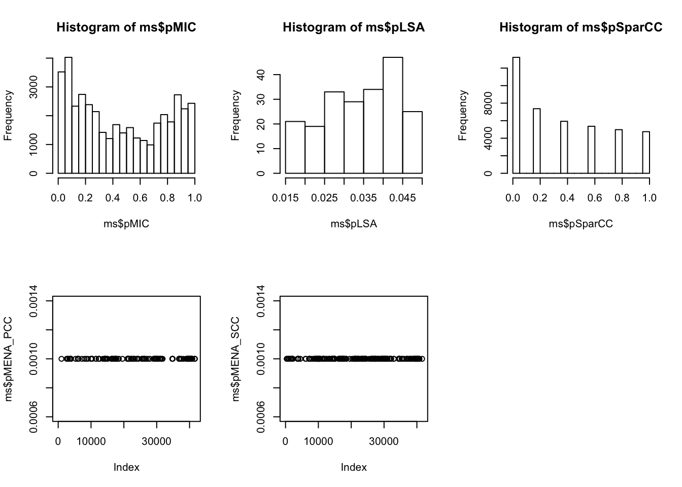

# metap::sumlog doesn't think 0 is a valid p-value, replace all zeros with small non-zero values, e.g. half-minimum
ms$pSparCC[ms$pSparCC == 0] <- 0.005
ms$pMIC[ms$pMIC == 0] <- 5e-04

ms["NA_count"] <- NA
ms["signif_0.05"] <- NA
ms["signif_0.001"] <- NA
ms["sumlog"] <- NA

n <- 0
k <- dim(ms)[1]
while (n < k) {
    n <- n + 1
    ms$NA_count[n] <- sum(is.na(ms[n, 3:7]))
    ms$signif_0.05[n] <- sum(ms[n, 3:7] <= 0.05, na.rm = T)
    ms$signif_0.001[n] <- sum(ms[n, 3:7] <= 0.001, na.rm = T)
    ifelse((ms$NA_count[n] <= 3), (ms$sumlog[n] <- sumlog(ms[n, 3:7][!is.na(ms[n, 3:7])])$p), NA)
}
rm(k, n)

ms["p.adjust_Bonferroni"] <- p.adjust(ms$sumlog, method = "bonferroni")
ms["p.adjust_FDR"] <- p.adjust(ms$sumlog, method = "fdr")  #aka Benjamini & Hochberg

par(mfrow = c(1, 3))
hist(ms$signif_0.05, main = "p-values <= 0.05", xlab = "Counts per edge ", breaks = c(0, 1, 2, 3, 4, 5), labels = TRUE)
hist(ms$signif_0.001, main = "p-values <= 0.001", xlab = "Counts per edge ", breaks = c(0, 1, 2, 3, 4, 5), labels = TRUE)
hist(ms$NA_count, main = "NAs", xlab = "Counts per edge ", breaks = c(0, 1, 2, 3, 4, 5), labels = TRUE)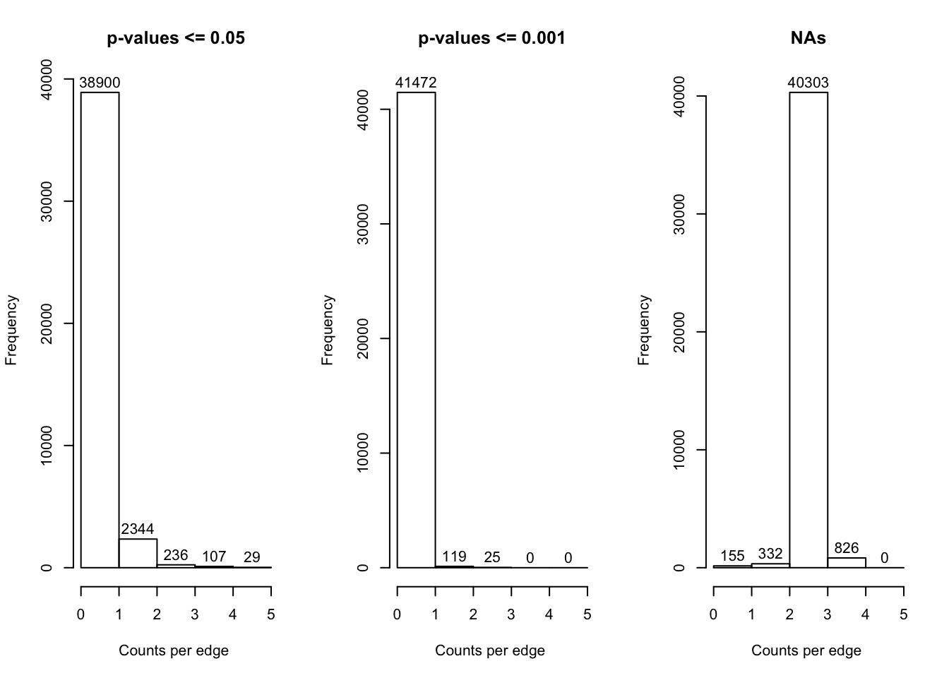

par(mfrow = c(1, 1))

ds <- split(ms, ms$signif_0.05)
raw_nodes <- rbind(ds$`4`, ds$`5`)  # Selection/inclusion criterion
rm(ds)

edges <- raw_nodes[, 1:2]
nodes <- union(raw_nodes$node1_mic, raw_nodes$node2_mic)

write.csv(edges, "data/master_summary_networks_2.csv", row.names = F)

We selected all edges with at least 4 p-values \(\leq\) 0.05 to visualise in the network. This consensus network has 136 edges and 113 nodes. Below are two versions of the network. In the first version, all OTUs correlating with barettin are colour-coded by class. In the second version, all OTUs increasing/decreasing woth depth are highlighted by colour.

# THANK YOU: https://kateto.net/networks-r-igraph

edges <- read.csv("data/master_summary_networks_2.csv", header = T, sep = ",")
nodes <- data.frame(union(raw_nodes$node1_mic, raw_nodes$node2_mic))

# annotation data required: inc-dec/depth response, taxonomy, barettin corelation hex color code
depth <- read.csv("data/gb_OTUs_overall_rabdc_annotated.csv", header = T, sep = ",")
taxonomy <- read.csv("data/microbiome_taxonomy.csv", header = T, sep = ";")
barettin <- read.csv("data/GB_OTU_barettin_correlation.csv", header = T, sep = ",")

# matching IDs
colnames(nodes) <- c("OTU_long")
nodes["OTU"] <- str_replace(nodes$OTU_long, "OTU196900", "")
depth["OTU"] <- str_replace(depth$XOTU, "X196900", "")
taxonomy["OTU"] <- str_replace(taxonomy$OTU_ID, "196900", "")
barettin["OTU"] <- str_replace(barettin$XOTU, "X196900", "")

# downsizing to relevant columns nodes$OTU_long <- NULL
depth <- depth[, c("ttest_pval", "ttest_fdr", "inc_dec_estimate", "inc_dec_p_val", "fdr", "classification", "OTU")]
colnames(depth) <- c("ttest_pval", "ttest_fdr", "inc_dec_estimate", "inc_dec_p_val", "inc_dec_fdr", "inc_dec_classification", "OTU")
barettin$XOTU <- NULL
taxonomy <- taxonomy[, c("Kingdom", "Phylum", "Class", "OTU")]
taxonomy[] <- lapply(taxonomy, str_trim)

nodes <- left_join(nodes, depth)
nodes <- left_join(nodes, barettin)
nodes <- left_join(nodes, taxonomy)

# Adding categorical information nodes['barettin_c'] <- ifelse(nodes$barettin_estimate_P>0 & nodes$barettin_p_val_P<0.05, 1, 0) # for scaling node size
nodes["barettin_c"] <- ifelse(nodes$barettin_p_val_P < 0.05, 1, 0)  # for scaling node size; both significant pos and neg this time
nodes["barettin_resp"] <- 0  # new: classifier for pos or neg barettin interaction
nodes$barettin_resp[nodes$barettin_c == 1 & nodes$barettin_estimate_P > 0] <- 1
nodes$barettin_resp[nodes$barettin_c == 1 & nodes$barettin_estimate_P < 0] <- 2
length(unique(nodes$Class[nodes$barettin_c == 1]))  #coloring by class impossible with 21different categories

## [1] 21

unique(nodes$Phylum[nodes$barettin_c == 1])  # use colors from rel abdc plot

## [1] "Acidobacteria"    "Thaumarchaeota"   "Proteobacteria"   "Chloroflexi"      ""                 "Gemmatimonadetes" "Nitrospirae"      "Actinobacteria"

nodes["OTU_lab"] <- c("")
nodes$OTU_lab[nodes$barettin_c == 1] <- nodes$OTU
nodes["inc_dec_c"] <- 0
nodes$inc_dec_c[nodes$inc_dec_p_val < 0.05] <- 1  # for scaling node size
nodes["inc_dec_c_group"] <- NA
nodes$inc_dec_c_group[nodes$inc_dec_c == 1 & nodes$inc_dec_estimate > 0] <- c("deep")  # for colouring shallow vs. deep
nodes$inc_dec_c_group[nodes$inc_dec_c == 1 & nodes$inc_dec_estimate < 0] <- c("shallow")  # for colouring shallow vs. deep
# Pearson pmcc > 0 & p < 0.05 56 fdr < 0.05 22 Spearman rho > 0 & p < 0.05 42 fdr < 0.05 1

nodes[] <- lapply(nodes, function(x) if (is.factor(x)) factor(x) else x)

library(igraph)
net <- graph_from_data_frame(d = edges, vertices = nodes, directed = F)
l <- layout_with_kk(net)

# 11 colourblind-friendly colours from https://medialab.github.io/iwanthue/

# Taxonomy coloring & barettin: Class ecol <- rep('gray80', ecount(net)) vcol <- rep('grey40', vcount(net)) vcol[V(net)$Class=='Subgroup_26'] <- '#628ed6'
# vcol[V(net)$Class=='Subgroup_15'] <- '#957d34' vcol[V(net)$Class=='Subgroup_6'] <- '#45c097' vcol[V(net)$Class=='Anaerolineae'] <- '#ba4758'
# vcol[V(net)$Class=='JG30-KF-CM66'] <- '#b2467e' vcol[V(net)$Class=='SAR202_clade'] <- '#5b3687' vcol[V(net)$Class=='TK10'] <- '#ba5437'
# vcol[V(net)$Class=='BD2-11_terrestrial_group'] <- '#69ab54' vcol[V(net)$Class=='Alphaproteobacteria'] <- '#c777cb' vcol[V(net)$Class=='JTB23'] <- '#c3a63e'
# vcol[V(net)$Class=='Acidimicrobiia'] <- '#6a70d7' colrs
# <-c('#628ed6','#957d34','#45c097','#ba4758','#b2467e','#5b3687','#ba5437','#69ab54','#c777cb','#c3a63e','#6a70d7') V(net)$color <- colrs[V(net)$Class]

# Taxonomy coloring & barettin: Phylum
ecol <- rep("gray80", ecount(net))
vcol <- rep("grey40", vcount(net))
vcol[V(net)$Phylum == "Acidobacteria"] <- "#b8c4f6"
vcol[V(net)$Phylum == "Thaumarchaeota"] <- "#aba900"
vcol[V(net)$Phylum == "Proteobacteria"] <- "#ff633f"
vcol[V(net)$Phylum == "Chloroflexi"] <- "#01559d"
vcol[V(net)$Phylum == "Gemmatimonadetes"] <- "#019c51"
vcol[V(net)$Phylum == "Nitrospirae"] <- "#49ca00"
vcol[V(net)$Phylum == "Actinobacteria"] <- "#ffaaaf"
vcol[V(net)$Phylum == ""] <- "#ffffff"
colrs <- c("#b8c4f6", "#aba900", "#ff633f", "#01559d", "#019c51", "#49ca00", "#ffaaaf", "#ffffff")
V(net)$color <- colrs[V(net)$Phylum]


V(net)$shape <- c("none", "circle", "csquare")[V(net)$barettin_resp + 1]

# set vertex.label=V(net)$OTU for OTU numbers
plot(net, vertex.color = vcol, edge.color = ecol, vertex.size = V(net)$barettin_c * 7, vertex.label = V(net)$OTU_lab, layout = l)
legend(x = 1, y = 0.5, c("Acidobacteria", "Thaumarchaeota", "Proteobacteria", "Chloroflexi", "Gemmatimonadetes", "Nitrospirae", "Actinobacteria", "unclasified"), 
    pt.bg = colrs, pch = 21, col = "#777777", pt.cex = 1.5, cex = 0.7, bty = "n", ncol = 1)

Figure 4.1: Microbial interaction networks highlighting OTUs correlating with barettin and OTUs correlating with depth.

# legend(x=1, y=0.5, c('Subgroup_26 (Acidobacteria)','Subgroup_15 (Acidobacteria)', 'Subgroup_6 (Acidobacteria)', 'Anaerolineae (Chloroflexi)', 'JG30-KF-CM66
# (Chloroflexi)', 'SAR202_clade (Chloroflexi)', 'TK10 (Chloroflexi)', 'BD2-11_terrestrial_group (Gemmatimonadetes)', 'Alphaproteobacteria (Proteobacteria)',
# 'JTB23 (Proteobacteria)', 'Acidimicrobiia (Actinobacteria)'), pt.bg=colrs, pch=21,col='#777777', pt.cex=1.5, cex=.7, bty='n', ncol=1)

# circles are positive correlations with barettin, squares are negative


# Depth by correlation
ecol <- rep("gray80", ecount(net))
vcol <- rep("grey40", vcount(net))
vcol[V(net)$inc_dec_c_group == "shallow"] <- "gold"
vcol[V(net)$inc_dec_c_group == "deep"] <- "blue"

V(net)$color <- colrs[V(net)$inc_dec_c_group]
colrs <- c("gold", "blue")

plot(net, vertex.color = vcol, edge.color = ecol, vertex.size = V(net)$inc_dec_c * 10, vertex.label = NA, layout = l)
legend(x = 1, y = 0.5, c("decreasing", "incerasing"), pt.bg = colrs, pch = 21, col = "#777777", pt.cex = 1.5, cex = 0.7, bty = "n", ncol = 1)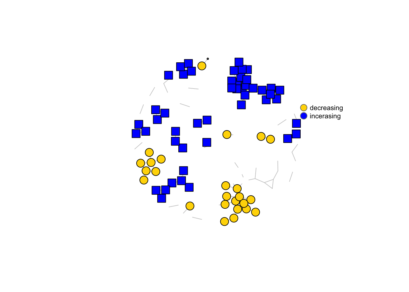

Figure 4.2: Microbial interaction networks highlighting OTUs correlating with barettin and OTUs correlating with depth.

4.4 Shortlist

We believe the producer of barettin (and related compounds) to have the following properties:

common (average relative abundance > 0.25%)
specific to G. barretti
positively correlated with barettin

the OTUs below fulfill these criteria:

# most annotation from NW
micro <- read.csv("data/OTU_all_R.csv", header = T, sep = ";")

OTU_prep_sqrt <- function(micro) {
    rownames(micro) <- micro$Sample_ID
    micro$Sample_ID <- NULL
    # micro <- sqrt(micro)
    
    micro_gb <- micro[(str_sub(rownames(micro), 1, 2) == "Gb"), ]
    micro_sf <- micro[(str_sub(rownames(micro), 1, 2) == "Sf"), ]
    micro_wb <- micro[(str_sub(rownames(micro), 1, 2) == "Wb"), ]
    
    micro_gb <- micro_gb[, colSums(micro_gb != 0) > 0]  #removes columns that only contain 0
    micro_sf <- micro_sf[, colSums(micro_sf != 0) > 0]
    micro_wb <- micro_wb[, colSums(micro_wb != 0) > 0]
    micros <- list(gb = micro_gb, sf = micro_sf, wb = micro_wb)
    return(micros)
}

micro_ds <- OTU_prep_sqrt(micro)

overall_rabdc <- function(micro) {
    mic <- micro
    n <- 0
    k <- dim(mic)[1]
    mic["rowsum"] <- apply(mic, 1, sum)
    
    while (n < k) {
        n <- n + 1
        mic[n, ] <- mic[n, ]/(mic$rowsum[n])
    }
    
    mic$rowsum <- NULL
    mic <- data.frame(t(mic))
    mic["avg_rel_abdc"] <- apply(mic, 1, mean)
    mic["occurrence"] <- ifelse(mic$avg > 0.0025, "common", "rare")
    return(mic)
}

occurrence <- lapply(micro_ds, overall_rabdc)

depth <- read.csv("data/gb_OTUs_overall_rabdc_annotated.csv", header = T, sep = ",")
taxonomy <- read.csv("data/microbiome_taxonomy.csv", header = T, sep = ";")
barettin <- read.csv("data/GB_OTU_barettin_correlation.csv", header = T, sep = ",")

# matching IDs
nodes["OTU"] <- str_replace(nodes$OTU_long, "OTU196900", "")
depth["OTU"] <- str_replace(depth$XOTU, "X196900", "")
taxonomy["OTU"] <- str_replace(taxonomy$OTU_ID, "196900", "")
barettin["OTU"] <- str_replace(barettin$XOTU, "X196900", "")
occurrence$gb["OTU"] <- str_replace(rownames(occurrence$gb), "X196900", "")

# downsizing to relevant columns nodes$OTU_long <- NULL
depth <- depth[, c("ttest_pval", "ttest_fdr", "inc_dec_estimate", "inc_dec_p_val", "fdr", "classification", "OTU")]
colnames(depth) <- c("ttest_pval", "ttest_fdr", "inc_dec_estimate", "inc_dec_p_val", "inc_dec_fdr", "inc_dec_classification", "OTU")
barettin$XOTU <- NULL
taxonomy[] <- lapply(taxonomy, str_trim)

# combining dfs
shortlist_gb <- left_join(occurrence$gb, depth)
shortlist_gb <- left_join(shortlist_gb, barettin)
shortlist_gb <- left_join(shortlist_gb, taxonomy)

# Exclude Sf OTUs intersect(colnames(micro_ds$gb), colnames(micro_ds$sf)) # shared OTUs length(intersect(colnames(micro_ds$gb), colnames(micro_ds$sf))) # 316

# setdiff(colnames(micro_ds$gb), colnames(micro_ds$sf)) # Setdiff finds rows that appear in first table but not in second
# length(setdiff(colnames(micro_ds$gb), colnames(micro_ds$sf))) # 104:ok!
gb_unique <- data.frame(setdiff(colnames(micro_ds$gb), colnames(micro_ds$sf)))
colnames(gb_unique) <- c("XOTU")
gb_unique["OTU"] <- str_replace(gb_unique$XOTU, "X196900", "")

gb_unique <- left_join(gb_unique, shortlist_gb)

gb_unique <- gb_unique %>% filter(occurrence == "common") %>% filter(barettin_estimate_P > 0 & barettin_p_val_P < 0.05)

# Recovery of those OTUs that also correlate with barettin in S. fortis
sf_shared <- data.frame(intersect(colnames(micro_ds$gb), colnames(micro_ds$sf)))
colnames(sf_shared) <- c("XOTU")
sf_barretin <- read.csv("data/SF_OTU_barettin_correlation.csv", header = T, sep = ",")

sf_shared <- left_join(sf_shared, sf_barretin)

# Sf Pearson p<0.05 24 pFDR>0.05 8 Spearman p<0.05 14 pFDR>0.05 0

sf_shared <- sf_shared %>% filter(barettin_estimate_P > 0) %>% filter(barettin_p_val_P < 0.05)

sf_shared["OTU"] <- str_replace(sf_shared$XOTU, "X196900", "")
shared_recovered <- shortlist_gb[shortlist_gb$OTU %in% sf_shared$OTU, ]

# check again for the criteria in the new df
shared_recovered <- shared_recovered %>% filter(occurrence == "common") %>% filter(barettin_estimate_P > 0 & barettin_p_val_P < 0.05)

# combine the two data sets: gb_unique and shared_recovered

gb_unique["group"] <- c("gb_unique")
shared_recovered["group"] <- c("sf_shared")

gb_unique <- gb_unique[, c("OTU", "group", "Kingdom", "Phylum", "Class")]
shared_recovered <- shared_recovered[, c("OTU", "group", "Kingdom", "Phylum", "Class")]

shortlist <- rbind(gb_unique, shared_recovered)

options(kableExtra.html.bsTable = T)
kable(shortlist, col.names = c("OTU", "group", "Kingdom", "Phylum", "Class"), longtable = T, booktabs = T, caption = "Shortlist of OTUs that were deemed candidate producers of barettin.", 
    row.names = FALSE) %>% add_header_above(c(` ` = 2, Taxonomy = 3)) %>% kable_styling(bootstrap_options = c("striped", "hover", "bordered", "condensed", "responsive"), 
    full_width = F, latex_options = c("striped", "scale_down"))

OTU	group	Kingdom	Phylum	Class
589	gb_unique	Bacteria	Chloroflexi	SAR202_clade
588	gb_unique	Bacteria	Acidobacteria	Subgroup_9
180	sf_shared	Bacteria	Proteobacteria	JTB23
144	sf_shared	Bacteria	Acidobacteria	Subgroup_9
213	sf_shared	Bacteria	Gemmatimonadetes	BD2-11_terrestrial_group
310	sf_shared	Bacteria	Proteobacteria	JTB23

micro <- read.csv("data/OTU_all_R.csv", header = T, sep = ";")
meta_data <- read.csv("data/Steffen_et_al_metadata_PANGAEA.csv", header = T, sep = ";")
cmp <- read.csv("data/metabolite_master_20190605.csv", header = T, sep = ",")

meta_data <- meta_data_prep(meta_data)

OTU_prep <- function(micro) {
    rownames(micro) <- micro$Sample_ID
    micro$Sample_ID <- NULL
    # micro <- sqrt(micro)
    
    micro_gb <- micro[(str_sub(rownames(micro), 1, 2) == "Gb"), ]
    micro_sf <- micro[(str_sub(rownames(micro), 1, 2) == "Sf"), ]
    micro_wb <- micro[(str_sub(rownames(micro), 1, 2) == "Wb"), ]
    
    micro_gb <- micro_gb[, colSums(micro_gb != 0) > 0]
    micro_sf <- micro_sf[, colSums(micro_sf != 0) > 0]
    micro_wb <- micro_wb[, colSums(micro_wb != 0) > 0]
    micros <- list(gb = micro_gb, sf = micro_sf, wb = micro_wb)
    return(micros)
}

micro_ds <- OTU_prep(micro)

overall_rabdc <- function(micros) {
    mic <- micros
    n <- 0
    k <- dim(mic)[1]
    mic["rowsum"] <- apply(mic, 1, sum)
    
    while (n < k) {
        n <- n + 1
        mic[n, ] <- mic[n, ]/(mic$rowsum[n])
    }
    
    mic$rowsum <- NULL
    mic <- data.frame(t(mic))
    # mic['avg_rel_abdc'] <- apply(mic, 1, mean) mic['occurrence'] <- ifelse(mic$avg>0.0025, 'common', 'rare')
    return(mic)
}

rabdc <- lapply(micro_ds, overall_rabdc)

rabdc$gb[, c("avg_rel_abdc", "occurrence")] <- list(NULL)

# Shortlist OTUs
sl <- rabdc$gb[c("X196900144", "X196900180", "X196900213", "X196900310", "X196900588", "X196900589"), ]
sl <- data.frame(t(sl))
sl["unified_ID"] <- rownames(sl)
sl <- left_join(sl, meta_data[, c("unified_ID", "Depth")])
sl <- left_join(sl, cmp[, c("unified_ID", "bar")])
summary(lm(X196900144 ~ bar, sl))

## 
## Call:
## lm(formula = X196900144 ~ bar, data = sl)
## 
## Residuals:
##       Min        1Q    Median        3Q       Max 
## -0.009272 -0.002497 -0.001386  0.002741  0.013684 
## 
## Coefficients:
##               Estimate Std. Error t value Pr(>|t|)    
## (Intercept) -3.026e-03  4.204e-03  -0.720  0.49218    
## bar          1.720e-08  2.992e-09   5.748  0.00043 ***
## ---
## Signif. codes:  0 '***' 0.001 '**' 0.01 '*' 0.05 '.' 0.1 ' ' 1
## 
## Residual standard error: 0.006446 on 8 degrees of freedom
##   (4 observations deleted due to missingness)
## Multiple R-squared:  0.8051, Adjusted R-squared:  0.7807 
## F-statistic: 33.04 on 1 and 8 DF,  p-value: 0.0004298

summary(lm(X196900180 ~ bar, sl))

## 
## Call:
## lm(formula = X196900180 ~ bar, data = sl)
## 
## Residuals:
##        Min         1Q     Median         3Q        Max 
## -0.0039199 -0.0014359 -0.0002769  0.0008649  0.0053601 
## 
## Coefficients:
##              Estimate Std. Error t value Pr(>|t|)    
## (Intercept) 9.756e-04  1.734e-03   0.562 0.589192    
## bar         6.287e-09  1.234e-09   5.093 0.000938 ***
## ---
## Signif. codes:  0 '***' 0.001 '**' 0.01 '*' 0.05 '.' 0.1 ' ' 1
## 
## Residual standard error: 0.002659 on 8 degrees of freedom
##   (4 observations deleted due to missingness)
## Multiple R-squared:  0.7643, Adjusted R-squared:  0.7348 
## F-statistic: 25.94 on 1 and 8 DF,  p-value: 0.0009383

summary(lm(X196900213 ~ bar, sl))

## 
## Call:
## lm(formula = X196900213 ~ bar, data = sl)
## 
## Residuals:
##        Min         1Q     Median         3Q        Max 
## -0.0031031 -0.0012324 -0.0004205  0.0011007  0.0048727 
## 
## Coefficients:
##               Estimate Std. Error t value Pr(>|t|)   
## (Intercept) -5.866e-04  1.642e-03  -0.357  0.73020   
## bar          3.927e-09  1.169e-09   3.360  0.00994 **
## ---
## Signif. codes:  0 '***' 0.001 '**' 0.01 '*' 0.05 '.' 0.1 ' ' 1
## 
## Residual standard error: 0.002518 on 8 degrees of freedom
##   (4 observations deleted due to missingness)
## Multiple R-squared:  0.5852, Adjusted R-squared:  0.5333 
## F-statistic: 11.29 on 1 and 8 DF,  p-value: 0.009939

summary(lm(X196900310 ~ bar, sl))

## 
## Call:
## lm(formula = X196900310 ~ bar, data = sl)
## 
## Residuals:
##        Min         1Q     Median         3Q        Max 
## -0.0023418 -0.0007641 -0.0005424 -0.0002813  0.0047438 
## 
## Coefficients:
##               Estimate Std. Error t value Pr(>|t|)  
## (Intercept) -9.181e-05  1.476e-03  -0.062   0.9519  
## bar          2.655e-09  1.051e-09   2.527   0.0354 *
## ---
## Signif. codes:  0 '***' 0.001 '**' 0.01 '*' 0.05 '.' 0.1 ' ' 1
## 
## Residual standard error: 0.002263 on 8 degrees of freedom
##   (4 observations deleted due to missingness)
## Multiple R-squared:  0.4439, Adjusted R-squared:  0.3744 
## F-statistic: 6.385 on 1 and 8 DF,  p-value: 0.03543

summary(lm(X196900588 ~ bar, sl))

## 
## Call:
## lm(formula = X196900588 ~ bar, data = sl)
## 
## Residuals:
##        Min         1Q     Median         3Q        Max 
## -0.0036391 -0.0008598 -0.0003235  0.0000593  0.0060071 
## 
## Coefficients:
##               Estimate Std. Error t value Pr(>|t|)  
## (Intercept) -5.362e-04  1.815e-03  -0.295    0.775  
## bar          2.997e-09  1.292e-09   2.320    0.049 *
## ---
## Signif. codes:  0 '***' 0.001 '**' 0.01 '*' 0.05 '.' 0.1 ' ' 1
## 
## Residual standard error: 0.002783 on 8 degrees of freedom
##   (4 observations deleted due to missingness)
## Multiple R-squared:  0.4021, Adjusted R-squared:  0.3274 
## F-statistic:  5.38 on 1 and 8 DF,  p-value: 0.04895

summary(lm(X196900589 ~ bar, sl))

## 
## Call:
## lm(formula = X196900589 ~ bar, data = sl)
## 
## Residuals:
##        Min         1Q     Median         3Q        Max 
## -0.0020026 -0.0004915 -0.0001909  0.0003738  0.0020246 
## 
## Coefficients:
##               Estimate Std. Error t value Pr(>|t|)    
## (Intercept) -3.725e-04  8.105e-04   -0.46  0.65800    
## bar          3.063e-09  5.769e-10    5.31  0.00072 ***
## ---
## Signif. codes:  0 '***' 0.001 '**' 0.01 '*' 0.05 '.' 0.1 ' ' 1
## 
## Residual standard error: 0.001243 on 8 degrees of freedom
##   (4 observations deleted due to missingness)
## Multiple R-squared:  0.779,  Adjusted R-squared:  0.7513 
## F-statistic: 28.19 on 1 and 8 DF,  p-value: 0.0007201

library(reshape2)
sl <- melt(sl, id.vars = c("unified_ID", "Depth", "bar"))
ggplot(sl, aes(x = Depth, y = value)) + geom_point() + facet_wrap(. ~ variable, scales = "free") + theme_bw() + scale_y_continuous(labels = scales::scientific) + 
    scale_x_continuous(labels = scales::scientific) + ggtitle("Shortlisted OTUs and depth")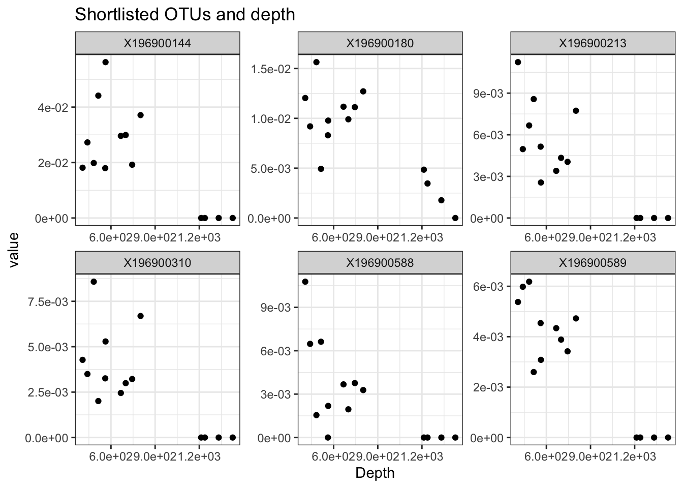

ggplot(sl, aes(x = bar, y = value)) + geom_point() + geom_smooth(method = "lm", formula = y ~ x) + facet_wrap(. ~ variable, scales = "free") + theme_bw() + theme(axis.text.x = element_text(angle = 90, 
    vjust = 0.5, hjust = 1)) + xlab("Barettin signal") + ylab("OTU relative abundance") + scale_y_continuous(labels = scales::scientific) + scale_x_continuous(labels = scales::scientific) + 
    ggtitle("Shortlisted OTUs and barettin")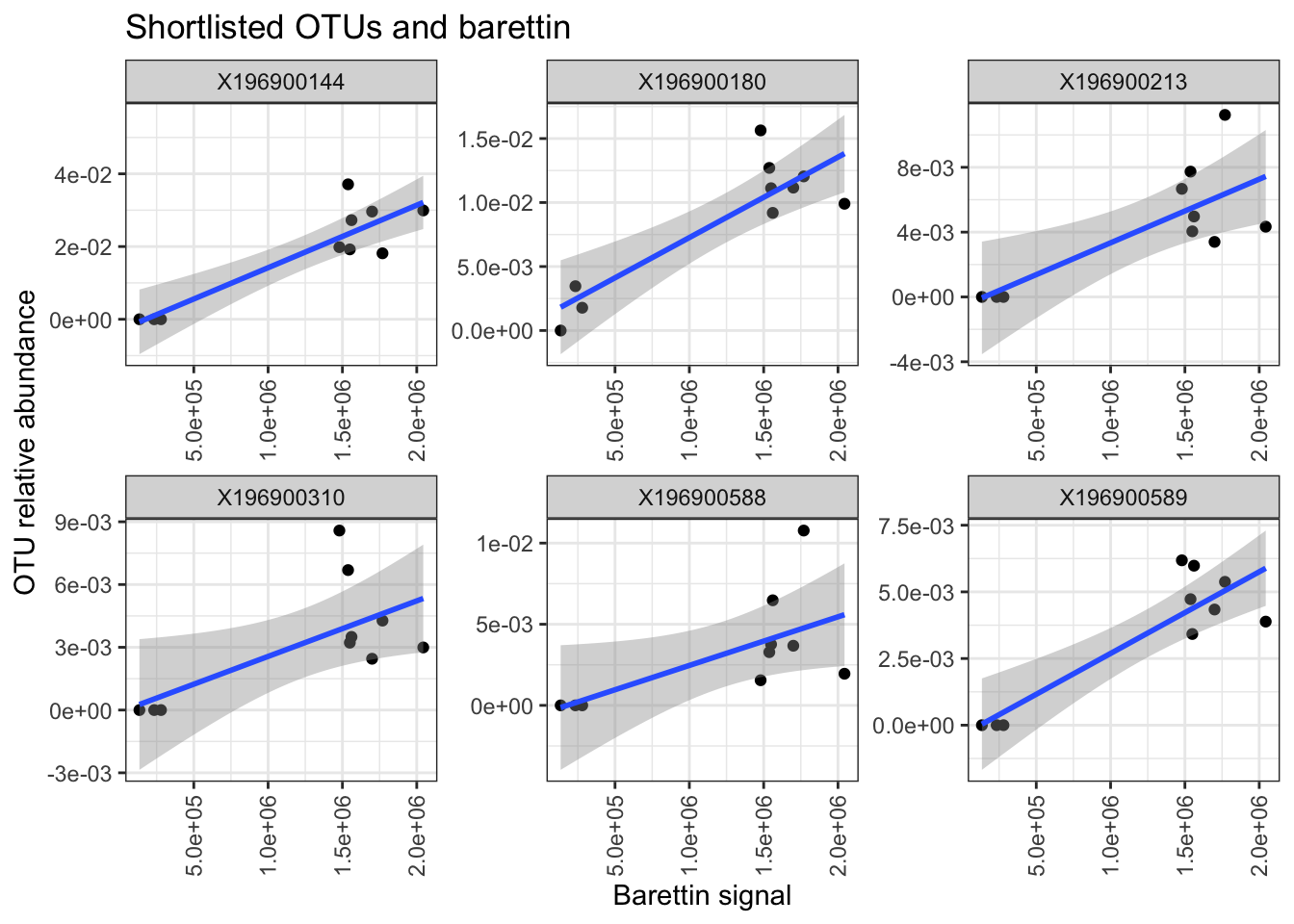

sessionInfo()

## R version 3.5.1 (2018-07-02)
## Platform: x86_64-apple-darwin15.6.0 (64-bit)
## Running under: macOS  10.15.5
## 
## Matrix products: default
## BLAS: /System/Library/Frameworks/Accelerate.framework/Versions/A/Frameworks/vecLib.framework/Versions/A/libBLAS.dylib
## LAPACK: /Library/Frameworks/R.framework/Versions/3.5/Resources/lib/libRlapack.dylib
## 
## locale:
## [1] en_US.UTF-8/en_US.UTF-8/en_US.UTF-8/C/en_US.UTF-8/en_US.UTF-8
## 
## attached base packages:
## [1] grid      stats     graphics  grDevices utils     datasets  methods   base     
## 
## other attached packages:
##  [1] minerva_1.5.8           viridis_0.5.1           viridisLite_0.3.0       pheatmap_1.0.12         rgl_0.100.50            plot3D_1.3             
##  [7] gtools_3.8.2            seqinr_3.6-1            picante_1.8.1           nlme_3.1-145            ape_5.3                 phyloseq_1.28.0        
## [13] DT_0.13                 RColorBrewer_1.1-2      ggExtra_0.9             plotly_4.9.2            ropls_1.14.1            reshape2_1.4.3         
## [19] usdm_1.1-18             raster_3.0-12           sp_1.4-1                rnaturalearthdata_0.1.0 rnaturalearth_0.1.0     sf_0.8-1               
## [25] marmap_1.0.3            mapdata_2.3.0           maps_3.3.0              ggmap_3.0.0.901         kableExtra_1.1.0.9000   gridExtra_2.3          
## [31] reshape_0.8.8           ggrepel_0.8.2           igraph_1.2.5            metap_1.3               vegan_2.5-6             lattice_0.20-41        
## [37] permute_0.9-5           forcats_0.5.0           stringr_1.4.0           dplyr_0.8.5             purrr_0.3.3             readr_1.3.1            
## [43] tidyr_1.0.2             tibble_3.0.0            ggplot2_3.3.0           tidyverse_1.3.0         knitr_1.28             
## 
## loaded via a namespace (and not attached):
##   [1] tidyselect_1.0.0        RSQLite_2.2.0           htmlwidgets_1.5.1       munsell_0.5.0           codetools_0.2-16        mutoss_0.1-12          
##   [7] units_0.6-6             miniUI_0.1.1.1          misc3d_0.8-4            withr_2.1.2             colorspace_1.4-1        Biobase_2.42.0         
##  [13] highr_0.8               rstudioapi_0.11         stats4_3.5.1            gbRd_0.4-11             Rdpack_0.11-1           labeling_0.3           
##  [19] RgoogleMaps_1.4.5.3     mnormt_1.5-6            bit64_0.9-7             farver_2.0.3            rhdf5_2.26.2            vctrs_0.2.4            
##  [25] generics_0.0.2          TH.data_1.0-10          xfun_0.13.1             R6_2.4.1                isoband_0.2.0           manipulateWidget_0.10.1
##  [31] bitops_1.0-6            assertthat_0.2.1        promises_1.1.0          scales_1.1.0            multcomp_1.4-12         rgeos_0.5-2            
##  [37] gtable_0.3.0            sandwich_2.5-1          rlang_0.4.5             splines_3.5.1           lazyeval_0.2.2          broom_0.5.5            
##  [43] yaml_2.2.1              modelr_0.1.6            crosstalk_1.1.0.1       backports_1.1.5         httpuv_1.5.2            tools_3.5.1            
##  [49] bookdown_0.18           ellipsis_0.3.0          biomformat_1.10.1       BiocGenerics_0.28.0     TFisher_0.2.0           Rcpp_1.0.4             
##  [55] plyr_1.8.6              zlibbioc_1.28.0         classInt_0.4-2          S4Vectors_0.20.1        zoo_1.8-7               haven_2.2.0            
##  [61] cluster_2.1.0           fs_1.4.0                magrittr_1.5            data.table_1.12.8       reprex_0.3.0            mvtnorm_1.1-0          
##  [67] hms_0.5.3               mime_0.9                evaluate_0.14           xtable_1.8-4            jpeg_0.1-8.1            readxl_1.3.1           
##  [73] IRanges_2.16.0          shape_1.4.4             compiler_3.5.1          KernSmooth_2.23-16      ncdf4_1.17              crayon_1.3.4           
##  [79] htmltools_0.4.0         mgcv_1.8-31             later_1.0.0             lubridate_1.7.4         DBI_1.1.0               formatR_1.7            
##  [85] dbplyr_1.4.2            MASS_7.3-51.5           Matrix_1.2-18           ade4_1.7-15             cli_2.0.2               parallel_3.5.1         
##  [91] pkgconfig_2.0.3         sn_1.6-1                numDeriv_2016.8-1.1     xml2_1.3.0              foreach_1.5.0           multtest_2.38.0        
##  [97] webshot_0.5.2           XVector_0.22.0          bibtex_0.4.2.2          rvest_0.3.5             digest_0.6.25           Biostrings_2.50.2      
## [103] rmarkdown_2.1           cellranger_1.1.0        shiny_1.4.0.2           rjson_0.2.20            lifecycle_0.2.0         jsonlite_1.6.1         
## [109] Rhdf5lib_1.4.3          fansi_0.4.1             pillar_1.4.3            fastmap_1.0.1           httr_1.4.1              plotrix_3.7-7          
## [115] survival_3.1-11         glue_1.3.2              png_0.1-7               iterators_1.0.12        bit_1.1-15.2            class_7.3-16           
## [121] adehabitatMA_0.3.14     stringi_1.4.6           blob_1.2.1              memoise_1.1.0           e1071_1.7-3